How to Flip Data in Excel Chart (5 Easy Methods)

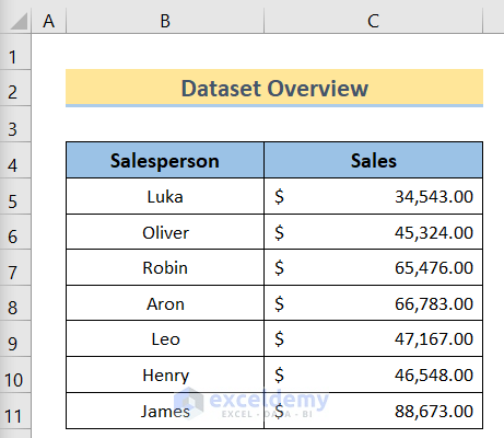
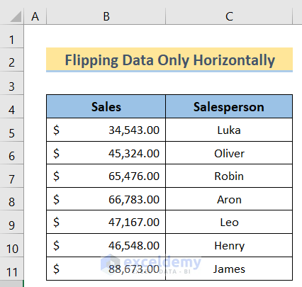
We’ll use a sample dataset with Salesperson in Column B and Sales in Column C. We’ll flip the data in the dataset.

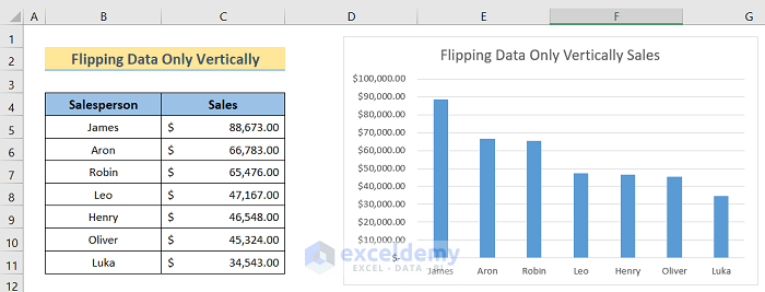
Method 1 – Flipping Data Only Vertically

Steps:

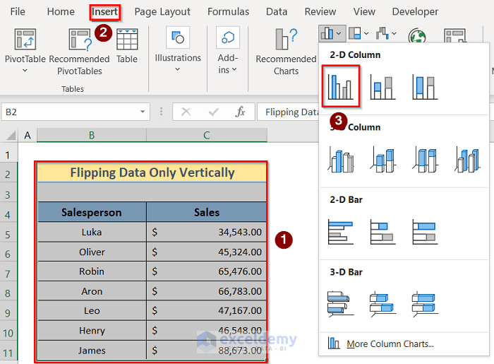
• Select the data.
• Go to Insert and select 2-D Column next to Charts to create a chart.

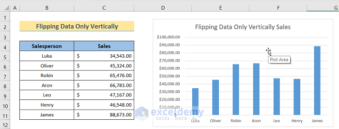
• You will get a chart.

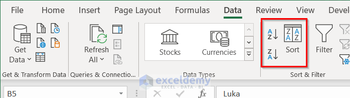
• Select the whole dataset and go to the Data tab.

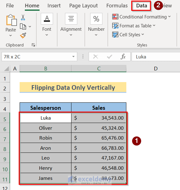
• In the Data tab, click on the Sort option.

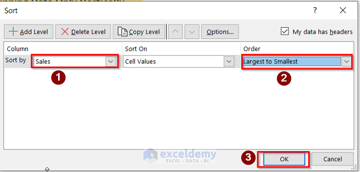
• The Sort dialog box will open on the screen.
• Select Sales in Sort by option and Largest to Smallest in Order option and press OK.

• You will get the desired result.

Read More: How to Flip Data Vertically in Excel

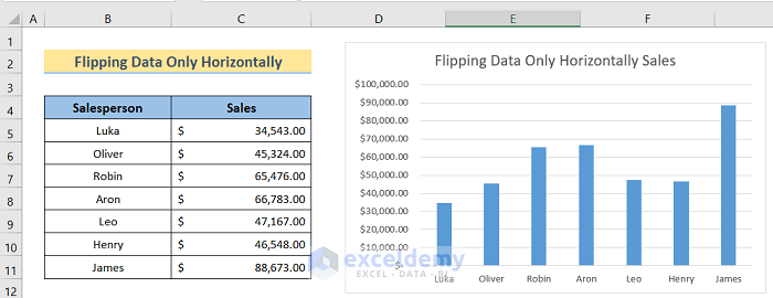
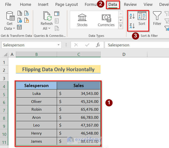
Method 2 – Flipping Data Only Horizontally

Steps:

• Create the data chart by following Method 1.

• Select the dataset.
• Go to Data and choose Sort.

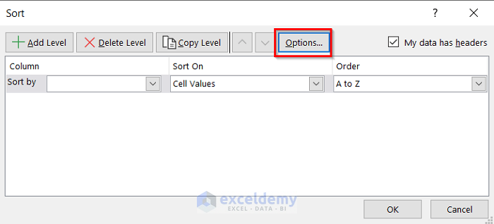
• The Sort dialog box will open. Click Options.

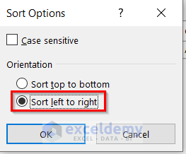
• Select the Sort left to right option in the dialog box and press OK.

• Select Row 4 in the Sort by option and press OK.

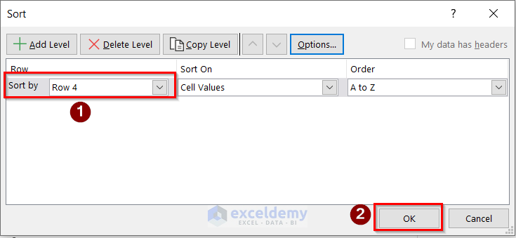
• You will get the desired result. You won’t get a graph in the chart.

Read More: How to Flip Data Horizontally in Excel

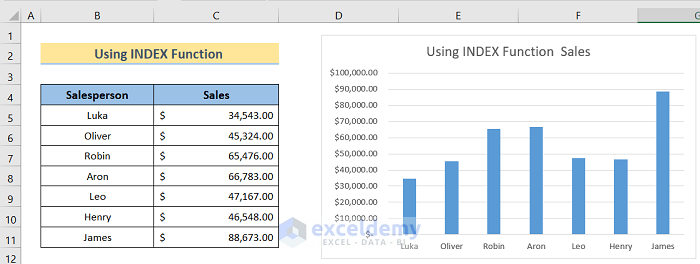
Method 3 – Using the INDEX Function

Steps:

• Create the data chart by following Method 1.

• Insert the following formula in cell E5.

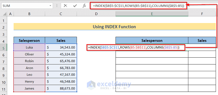
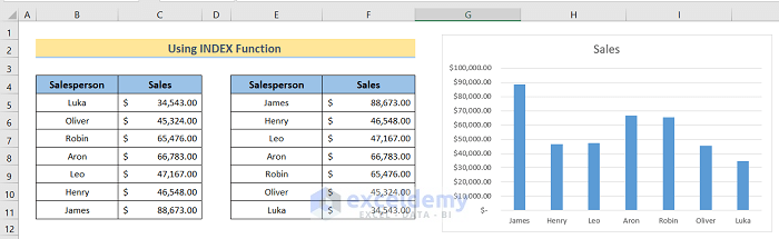
• Press Enter to get the desired result.

Method 4 – Use the SORTBY Function

If you are using Microsoft 365 then, you will get an extra option called the SORTBY Function.

Steps:

• Create the data chart by following Method 1.

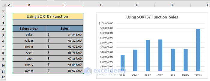
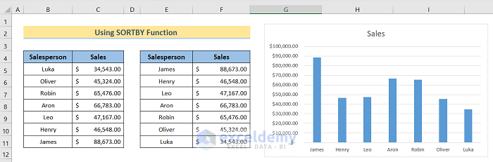
• Insert the following formula in cell E5.

• Press Enter to get the desired result.

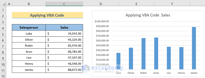
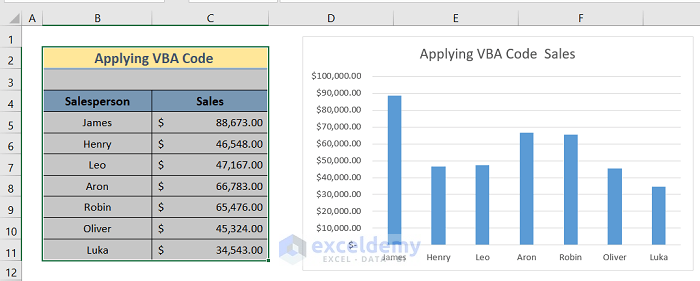
Method 5 – Applying VBA Code

Steps:

• Create the data chart via Method 1.

• Press Ctrl + F11 to open the VBA window and go to the Insert and Module options.

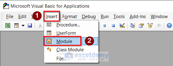
• Insert the following code in the window.

Sub FlipData()
Dim TRw As Variant
Dim LstRw As Variant
Dim SrtNum As Integer
Dim LstNum As Integer
Application.ScreenUpdating = False
SrtNum = 1
LstNum = Selection.Rows.Count
Do While SrtNum < LstNum
TRw = Selection.Rows(SrtNum)
LstRw = Selection.Rows(LstNum)
Selection.Rows(LstNum) = TRw
Selection.Rows(SrtNum) = LstRw
SrtNum = SrtNum + 1
LstNum = LstNum - 1
Loop
Application.ScreenUpdating = True
End Sub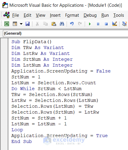

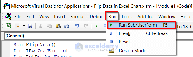
• Press Run.

• You will get the desired result.

How to Reverse an Axis in Excel Chart

Steps:

• Select the data.
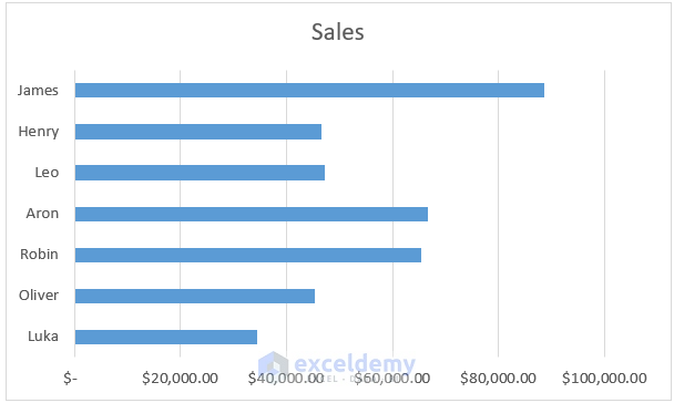
• Go to Insert and select 2-D Bar Chart.

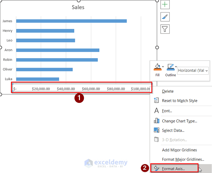
• You will get a chart.

• Right-click on the y-axis of the chart and select the Format Axis option.

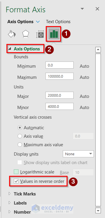
• The Format Axis dialog will open. Select the Values in reverse order option from the Axis Options.

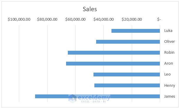
• You will get the desired result.

Things to Remember

• In the first two methods, we have flipped the data only vertically and horizontally individually. So, these methods are helpful while flipping data to one side only.
• When using the INDEX Function, you have to be careful about selecting cells.
• The SORTBY Function is only available for Microsoft 365 users.
• Using VBA code is the most efficient way among all the methods, but requires advanced knowledge of VBA to fix issues.

Download the Practice Workbook

Related Article

• How to Flip Table in Excel
• How to Mirror Data in Excel
• How to Reverse Text to Columns in Excel
• How to Reverse Column Order in Excel
• How to Reverse Data in Excel Chart

<< Go Back to Excel Reverse Order | Sort in Excel | Learn Excel