How to Reverse Text to Columns in Excel (6 Handy Methods)

This article provides the answer to the question of how to reverse Text to Columns in Excel. If you are looking for such unique tricks to do this, you’ve come to the right place. Here, we will take you through 6 easy and convenient methods for reversing text to columns in Excel.
For clarification, we’ll merge the two adjacent columns into a single column. The text strings in those two columns will get merged and displayed in the new column.
This is the reverse operation of the Text to Columns feature of Excel.

What Is Text to Columns Feature in Excel?

Before going into the details, let’s dwell a little upon what is Text to Columns feature in Excel is. The Text to Columns feature in Excel is very powerful if you want to separate your dataset into different columns. This can also help to move text from one column to the other. This feature becomes very useful when you change your mind regarding how your data should be organized.

How to Reverse Text to Columns in Excel: 6 Handy Methods

Already, you’ve know about the Text to Columns feature in Excel in the above section. In this portion, we’ll show how to reverse the Text to Columns feature in Excel.
To clarify the approach, we are using a Name List of Students. This dataset contains the First Names and Last Names of some students of a certain institution.

Now, we’ll combine the text strings of these two columns and show them in a single column only. Let’s explore these methods one by one.
Here, we have used Microsoft Excel 365 version, you may use any other version according to your convenience.

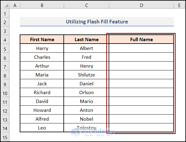
1. Utilizing Flash Fill Feature to Reverse Text to Columns in Excel

In the first method, we’ll use the Flash Fill feature of Excel. We can easily reverse Text to Columns using this tool. To do this using the first method, you may follow the below steps.

📌 Steps:

• At the very beginning, create a new column at the right of the Last Name column.
• Also, name it as Full Name.

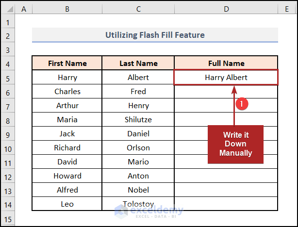
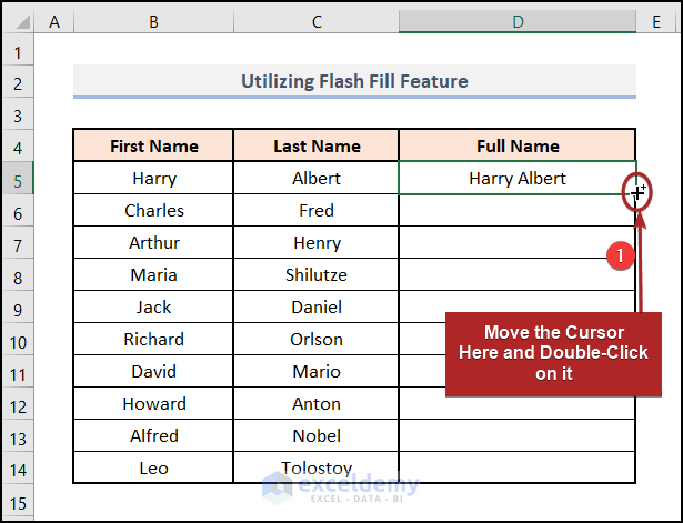
• Then, select cell D5 and write down Harry Albert manually.
• Actually, it’s his Full Name containing the First and Last Name.

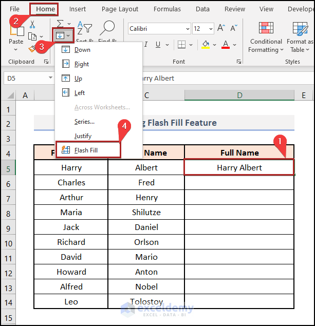
• At this moment, select cell D5.
• Secondly, go to the Home tab.
• Thirdly, click on the Fill drop-down icon on the Editing group.
• Fourthly, select Flash Fill from the options.

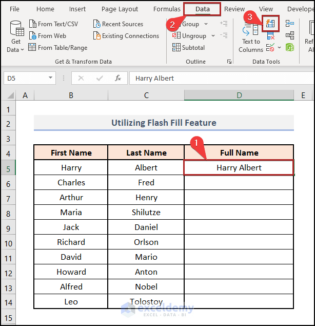
There is another way to call the Flash Fill feature. Just see the following steps.

• At first, select cell D5.
• Then, move to the Data tab.
• After that, select Flash Fill icon on the Data Tools group.
• Alternatively, press CTRL+E to do the same task.

For those of you who want to learn about more techniques, there is another one also. Don’t be surprised. Just follow along.

• Firstly, use your mouse to place the cursor on the right-bottom corner of the selected cell D5.
• Then, double-click on it.

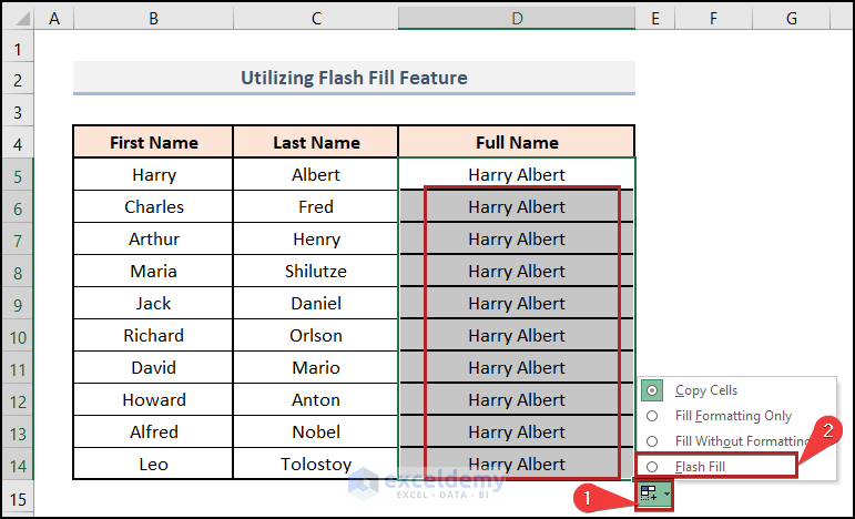
• The remaining cells get filled with Harry Albert by your previous action.
• Now, click on the Auto Fill Options icon at the end of the cells.
• Then, choose Flash Fill from the options.

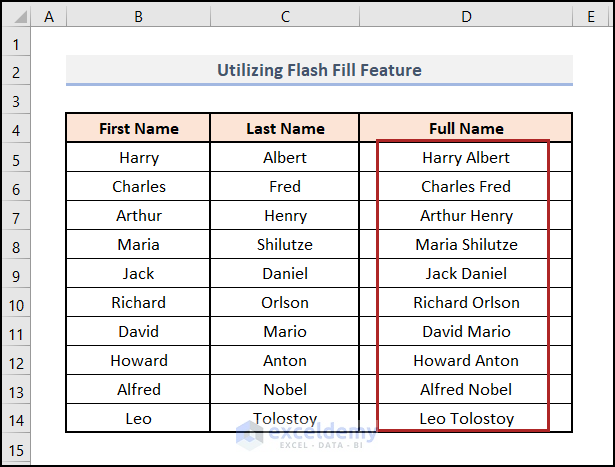
• Thus, you’ll get the Full Names in the remaining cells using any one of the three approaches stated above.

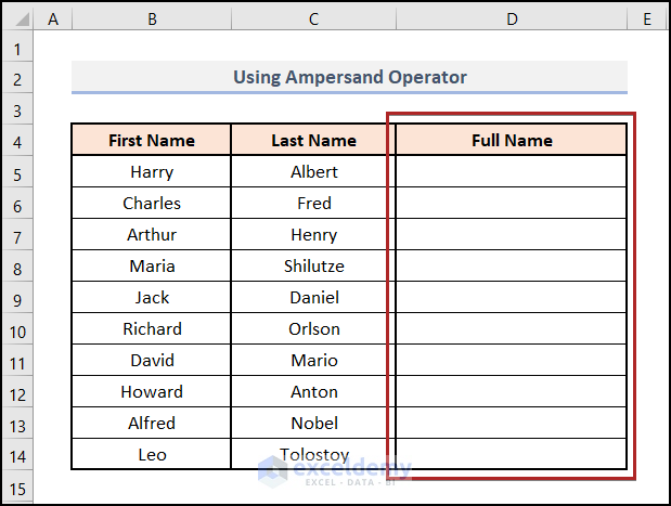
2. Using Ampersand (&) Operator to Reverse Text to Columns in Excel

If you’re one of those people who enjoy using Excel formulas then our next 3 methods have you covered. Particularly, in this method, we are going to discuss the use of the Ampersand (&) operator to reverse Text to Columns in Excel. Let’s explore the method step by step.

📌 Steps:

• At first, create a new column Full Name just like Method 1.

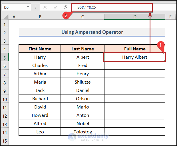
• After that, select cell D5 and write down the following formula in the Formula Bar.

Here, B5 and C5 represent the First Name and Last Name of the first student. We used a blank space between two Ampersand operators. Hence, it creates a gap between the two parts of the name.

• Then, press ENTER.

• At this time, move the cursor as shown in the image below. It will show the Fill Handle tool.
• Later, double-click on the mouse.

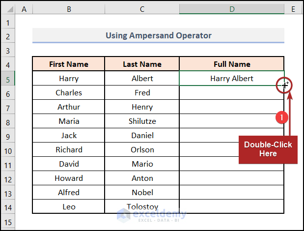
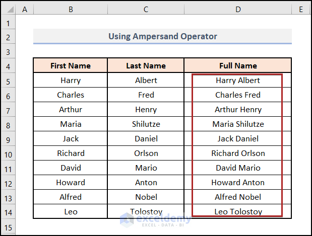
• Thus, it makes the remaining cells get filled with the results.

Read More: How to Reverse Column Order in Excel

3. Implementing CONCAT Function

In this method, we will use the CONCAT function in our formula. Let’s see the process in detail.

📌 Steps:

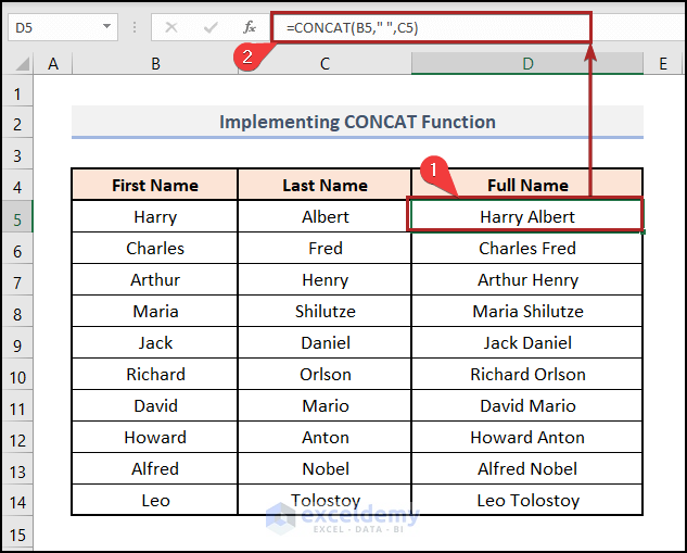
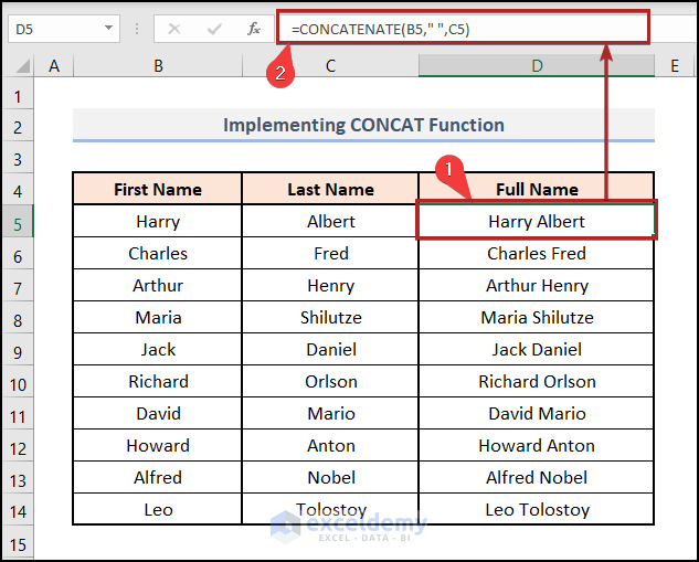
• Initially, select cell D5 and paste the following formula.

• Secondarily, press the ENTER key.

For doing this task, we can also use the old CONCATENATE function. The process is entirely similar to the above approach.

• Just select cell D5 and put the formula below.

• As always, hit the ENTER key.

4. Employing TEXTJOIN Function to Reverse Text to Columns in Excel

When you have a tool like Microsoft Excel, you can effortlessly perform a task in numerous ways. Here, we’ll use the TEXTJOIN function. So, without further delay, let’s dive in!

📌 Steps:

• Primarily, select cell D5 and put the following formula.

• Steadily, tap ENTER.

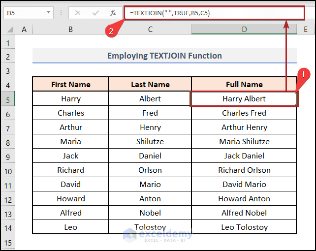
Then, we used the Fill Handle tool to get the other results.

5. Executing Power Query to Reverse Text to Columns in Excel

Are you looking for any antithetic way to do the same task? Then, you’re in the right hand. Now we’ll use Power Query to solve the problem. So, allow me to demonstrate the process below.

📌 Steps:

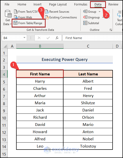
• In the first place, select cell B4. You can any other cell inside the data range.
• Secondly, jump to the Data tab.
• Thirdly, select From Table/Range on the Get & Transform Data group.

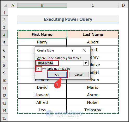
• Suddenly, the Create Table dialog box opens.
• Here, we can see that the range of cells gets automatically detected by Excel.
• Then, make sure that the box of My table has headers gets checked.
• Lastly, click OK.

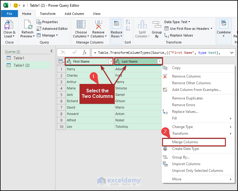
• At this moment, we can see the columns open in the Power Query Editor.
• Then, select the two columns using the CTRL key.
• After that, right-click on the column heading area.
• Later, select Merge Columns from the context menu.

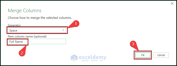
• Next, the Merge Columns wizard opens.
• Here, choose Space as Separator.
• Also, give a New column name. In this case, we named it as Full Name.
• Lastly, click OK.

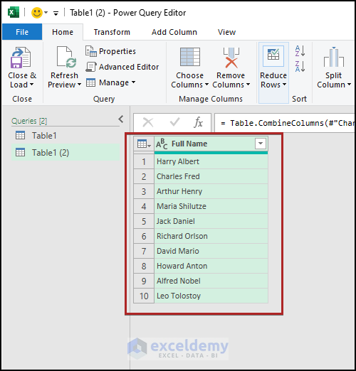
• Hence, we could successfully merge the two columns.

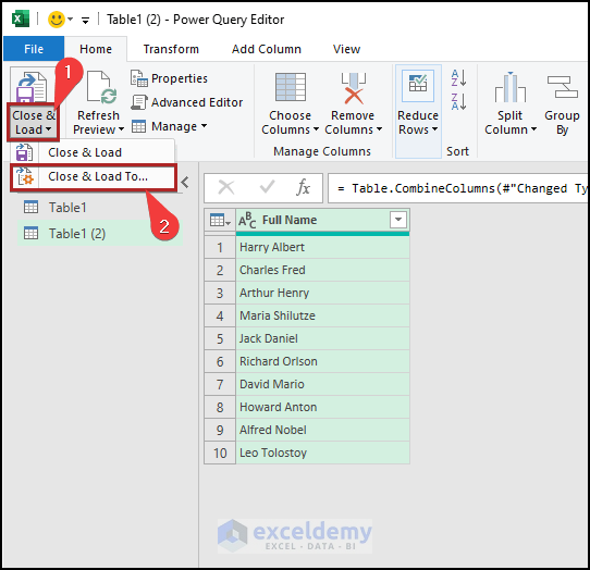
• In this instance, go to the Home tab.
• Then, click on the Close & Load drop-down.
• After that, select Close & Load To from the two options.

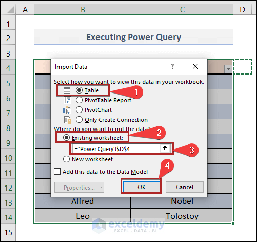
• Immediately, the Import Data wizard will open.
• Here, select Table under the Select how you want to view that data in your workbook section.
• Then, choose the Existing worksheet under Where do you want to put the data? section.
• Also, give the cell reference of D4 in the input box.
• Lastly, click OK.

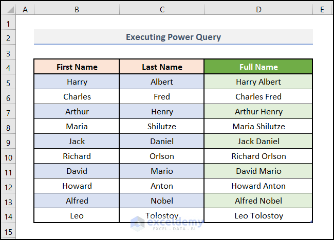
• The merged column is now available in our worksheet Power Query.

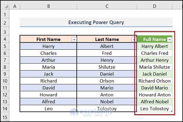
• Subsequently, do some formatting stuff and the worksheet will look like the one below.

Read More: How to Reverse Order of Columns Vertically in Excel

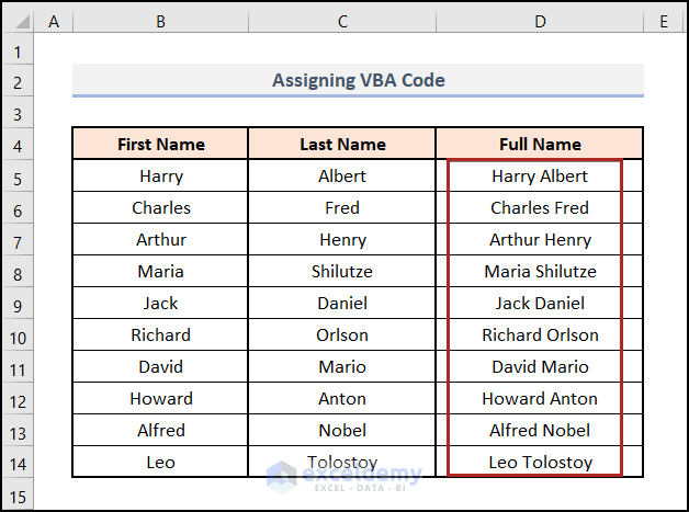
6. Assigning VBA Code

Although using formulas is a quick way of editing data, it can be difficult to interpret. Furthermore, if you often need to go the extra mile, then you may consider the VBA code below.

📌 Steps:

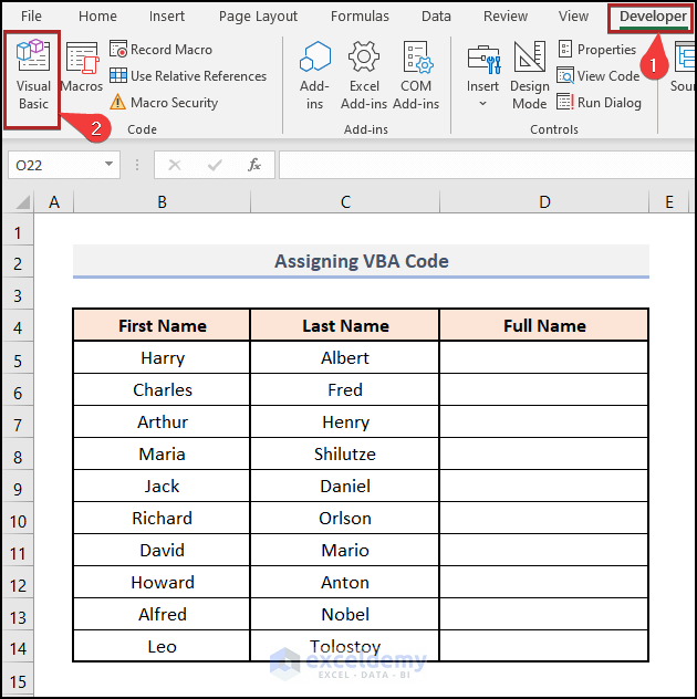
• Firstly, go to the Developer tab. If you can’t find it, then follow this link to display the Developer tab on the ribbon.
• Then, select Visual Basic on the Code group.
• Alternatively, press ALT+F11 to do the same task.

• Instantly, the Microsoft Visual Basic for Applications window opens.
• Afterward, move to the Insert tab.
• Later, select Module from the options.

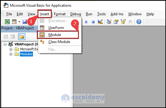
• Immediately, it opens the Code Module.
• Then, write down the following code in the Module.

Public Function Rvrs_Txt_Clmn(rng As Range, Optional S As String = " ") _
As String
Dim trns
trns = Application.WorksheetFunction.Transpose _
(Application.WorksheetFunction.Transpose(rng.Value))
Rvrs_Txt_Clmn = Join(trns, S)
End Function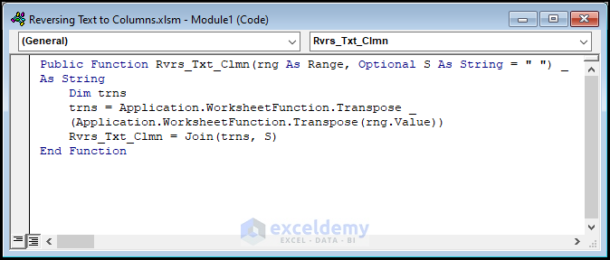

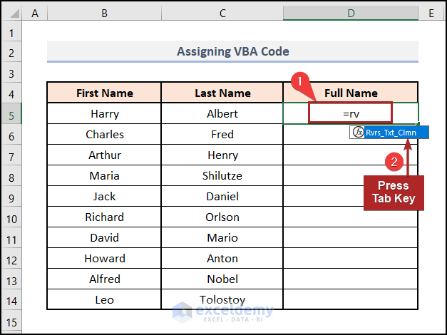
• Then, select cell D5 and write down =rv. Hence, we can see the function name in the suggestion.
• After that, press the Tab key to get the function working.

• Later, get the following formula into the cell.

Here, the Rvrs_Txt_Clmn is a public function. We’ve created this function just now.

• Correspondingly, hit ENTER.

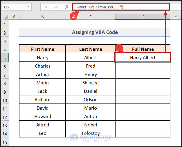
• Lastly, use the Fill Handle tool to get the full results like in the one below.

Practice Section

For doing practice by yourself we have provided a practice section like below in each sheet on the right side. Please do it by yourself.

Download Practice Workbook

You may download the following Excel workbook for better understanding and practice yourself.

Conclusion

This article provides easy and brief solutions to reverse Text to Columns in Excel. Don’t forget to download the Practice file. Thank you for reading this article, we hope this was helpful. Please let us know in the comment section if you have any queries or suggestions.

Related Articles

• How to Reverse Data in Excel Cell
• How to Mirror Data in Excel
• How to Reverse Order of Data in Excel
• How to Reverse Data in Excel Chart

<< Go Back to Excel Reverse Order | Sort in Excel | Learn Excel