Method 1 – Transposing Rows to Columns, Then Reversing Columns to Rows
Steps:
- Select the rows you want to reverse and copy it by pressing CTRL+C.
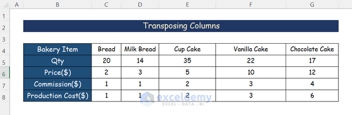
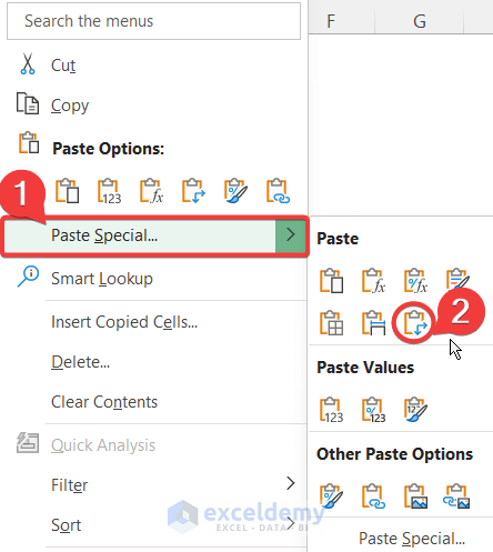
- Paste it using the Paste Special option by selecting Transpose from the Paste Special command.
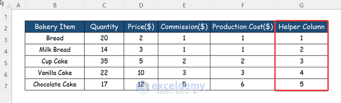
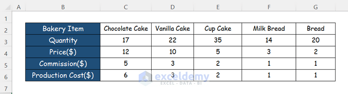
The selected rows will turn into columns as shown below.
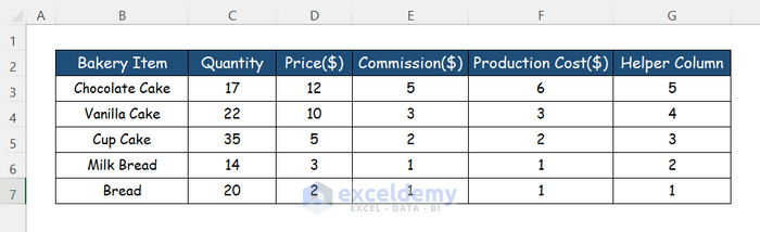
- Add a Helper column containing numbers 1, 2, 3, in sequence.
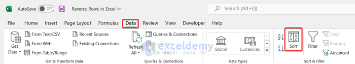
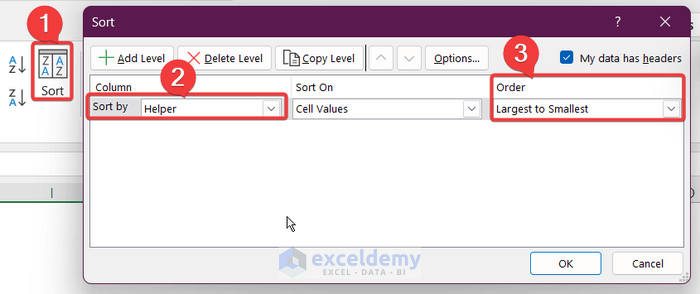
- Select all the columns, navigate to Data, and click on Sort.
A new window will open.
- Select Helper from the Sort by drop-down list. Click Largest to Smallest from the Order drop-down menu.
The data stored in the columns will be reversed.
- Delete the Helper Column.
- Transpose the columns back to rows by using the Transpose from Paste Special options as shown in step 2.
Read More: How to Paste in Reverse Order in Excel
Method 2 – Using Sort Feature to Reverse Rows in Excel
Steps:
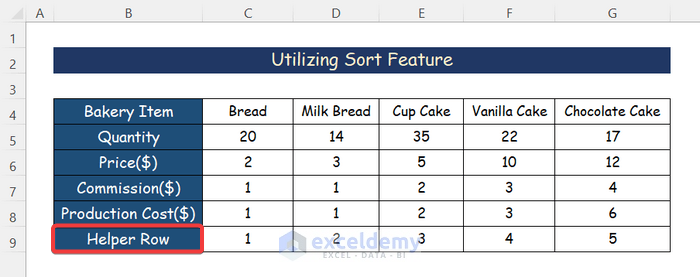
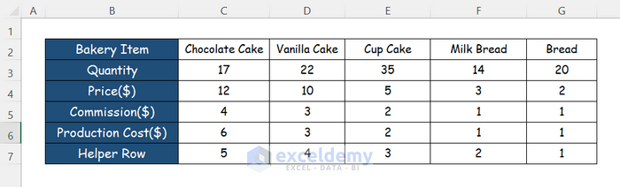
- Add a Helper Row with sequential numbers below the given rows.
- Select the complete data set including Helper Row.
- Click on the Data tab and click on Sort.
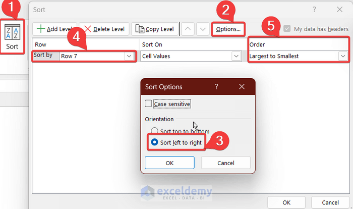
- From the Sort dialog box, click on Options and select Sort Left to Right.
- Press OK and select the Helper Row (row 7) number from the Sort by drop down menu.
- Select Largest to Smallest from the Order drop-down menu and click on OK.
The rows will be reversed horizontally.
- Delete the Helper Row.
Method 3 – Combining INDEX and COUNTA Functions to Reverse Rows
Steps:
- Select a cell outside the given data.
- Enter the following formula.
=INDEX($C$4:$G$4,1,COUNTA(C4:G4))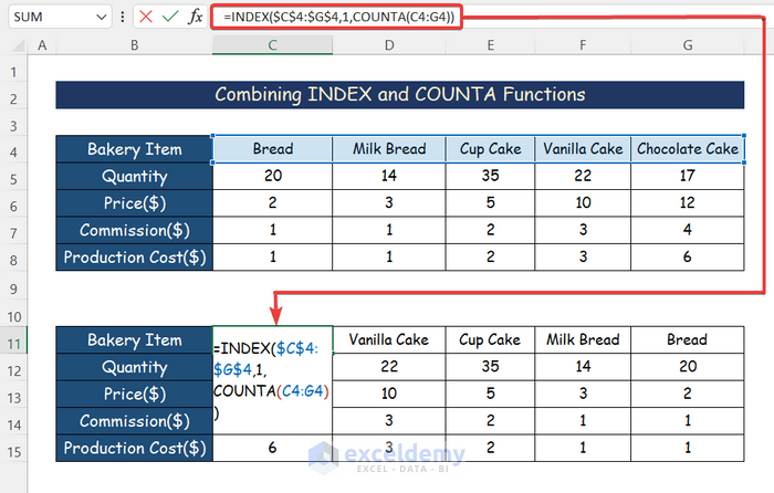
Formula Breakdown
- The COUNTA function counts all the non-blank cells within the range C4:G4.
- The INDEX function returns a value of the cell at the intersection of a particular row and column in a given range which includes 3 parts. It takes input value as an array within the range C4:G4, 1 is the row number and the column number is the output of the previous COUNTA
This will provide the reverse data.
- Select the cell and apply the AutoFill tool to the entire row in order to get the reverse data of the whole row.
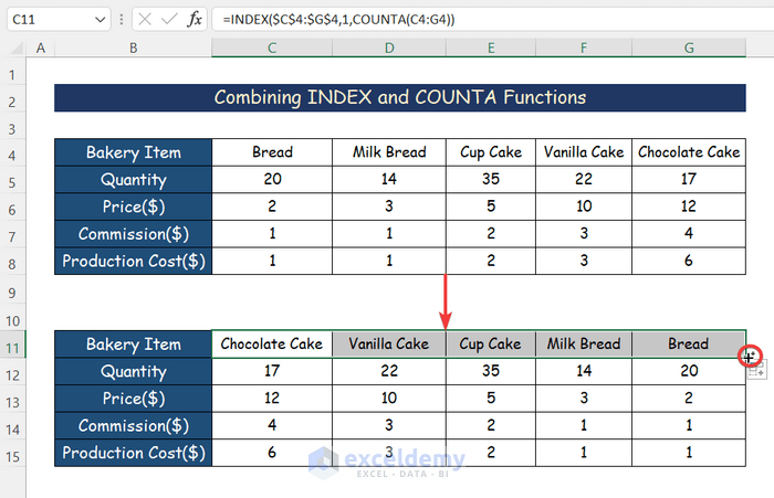
You can change the cell numbers in the formula and get the reversed rows.
Method 4 – Applying VBA to Reverse Rows in Excel
Steps:
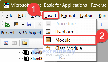
- Press Alt+F11 to open Microsoft Visual Basic Applications.
- Go to the Insert tab.
- Click on Module from the menu to create a module.
A new window will open.
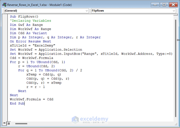
- Enter the following VBA macro in the Module.
Sub FlipRows()
‘ExcelDemy Publications
'Declaring Variables
Dim Gwf As Range
Dim WorkGwf As Range
Dim Cdd As Variant
Dim p As Integer, q As Integer, r As Integer
On Error Resume Next
xTitleId = "ExcelDemy"
Set WorkGwf = Application.Selection
Set WorkGwf = Application.InputBox("Range", xTitleId, WorkGwf.Address, Type:=8)
Cdd = WorkGwf.Formula
‘Applied For loop
For p = 1 To UBound(Cdd, 1)
    r = UBound(Cdd, 2)
    For q = 1 To UBound(Cdd, 2) / 2
        xTemp = Cdd(p, q)
        Cdd(p, q) = Cdd(p, r)
        Cdd(p, r) = xTemp
        r = r - 1
    Next
Next
WorkGwf.Formula = Cdd
End Sub
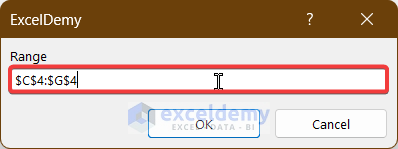
- Press F5 key to run the VBA.
A dialog box will open to select a range of rows.
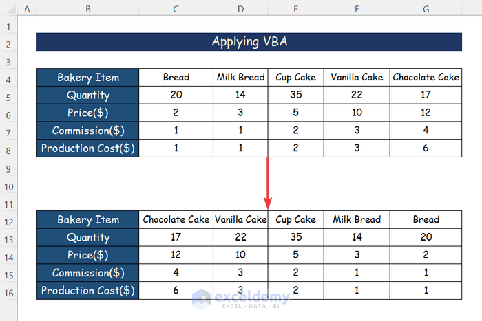
- Select the Range you want to reverse and press OK.
All the rows will be reversed horizontally.
Read More: How to Use Excel VBA to Reverse String
Download Practice Workbook
Related Articles
- How to Reverse a String in Excel
- How to Reverse a Number in Excel
- How to Reverse Names in Excel
- How to Switch First and Last Name in Excel with Comma
<< Go Back to Excel Reverse Order | Sort in Excel | Learn Excel
Get FREE Advanced Excel Exercises with Solutions!
