Method 1 – Using MID and CONCATENATE Functions to Reverse a String in Excel
Steps:
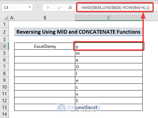
- Enter the following formula in cell C4:
=MID($B$4,LEN($B$4)-ROW(B4)+4,1)- The letter “y” should be returned as it is the last character in the provided string.
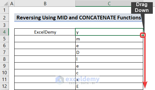
- Dag the fill handle downward, identical to the picture that is situated at the bottom right of cell C4.
- Enter the TRANSPOSE function in the cell that follows the final cell of column C, or cell C12, drag and select cells C4 through C12 before closing the parentheses around the TRANSPOSE formula.
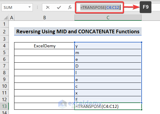
- Press F9 after selecting the entire formula in the formula bar. Then the formula bar will be like this:
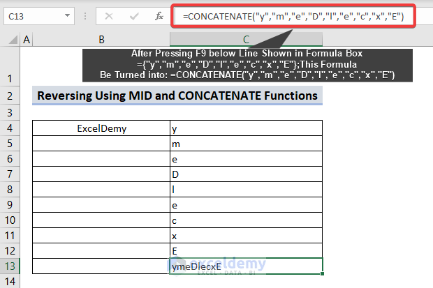
={"y","m","e","D","l","e","c","x","E"} - As our purpose is to use the CONCATENATE function, we will use this function after replacing the first curly brace and removing the second curly brace with the second parenthesis. This will turn into “ExcelDemy” to “ymeDlecxE”.
Method 2 – Reversing a String with MID and TEXTJOIN Functions
Steps:
- Insert the following formula in cell C4 and drag the fill handle to the last cell.
=TEXTJOIN("",1,MID(B4,{20,19,18,17,16,15,14,13,12,11,10,9,8,7,6,5,4,3,2,1},1))- The main purpose of this formula is to reverse strings like reversing the order of numbers in the array. The MID function returns a single character for each number in the array. TEXTJOIN joins those strings in reverse order.
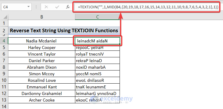
Note:
Only text with 20 characters or fewer than 20 characters can be used in this formula. But for longer strings, you have to use the VBA code below.
Method 3 – Applying VBA Code to Reverse a String in Excel
3.1 Apply VBA Code to a Single Cell
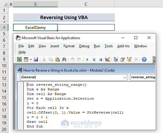
- By selecting the string that we want to reverse, we will press ALT+F11. The VBA window will appear. Copy the following string and paste it into the window.
Sub Reverse_String()
Dim s As Range
Set s = Application.Selection
s.Offset(0, 1).Value = StrReverse(s)
End Sub- Press F5 to run the VBA code. The result shown in the worksheet will be like “ymeDlecxE”.
3.2 Apply VBA Code to Multiple Cells
Steps:
- Pick the strings that we wish to reverse and tap ALT+F11, the VBA window will appear. We’ll copy the following VBA code and paste it into the window. To run the code press F5.
Sub reverse_string_range()
Dim s As Range
Dim cell As Range
Set s = Application.Selection
i = 0
For Each cell In s
cell.Offset(0, 1).Value = StrReverse(cell)
i = i + 1
Next cell
End Sub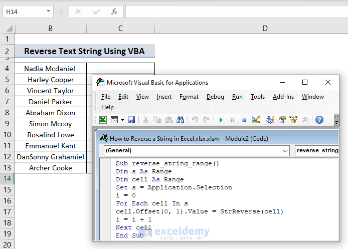
Download Practice Workbook
You can download the practice workbook from the following download button.
Related Articles
- How to Reverse Names in Excel
- How to Switch First and Last Name in Excel with Comma
- How to Paste in Reverse Order in Excel
- How to Reverse Rows in Excel
<< Go Back to Excel Reverse Order | Sort in Excel | Learn Excel
Get FREE Advanced Excel Exercises with Solutions!


A more elegant method:
A recursive Lambda function:
1) open “Name Manager”, click “New”
2) In “Name” type “RevText”
3) In “Refers to” type =LAMBDA(text,int, IF(int=0, “”, MID(text, int, 1) & RevText(text, int-1)))
You can now use “RevText” as a function, taking the text you want to reverse and the length of the text as parameters, like
=RevText(D50, LEN(D50))
Essentially what this does is set up a function that takes the last letter using a MID function, then feeds the results into itself, counting down the length of the text to zero)
Hello Sam Gardner,
That’s a great suggestion! Using a recursive Lambda function to reverse a string in Excel is indeed an elegant and efficient approach.
By setting up the function through the Name Manager, you can call it easily with any text and its length as parameters. It eliminates the need for complex formulas, making the process smoother.
Thanks for sharing this method!
Regards
ExcelDemy