How to Reverse Order of Data in Excel (4 Useful Methods)

In Excel, you might occasionally need to reverse the order of data, which means reversing the data order from left to right in a horizontal dataset and also inverting data upside down in a vertical dataset. There are various easy ways in Excel to do so. In this article, we are going to see some useful methods to reverse the order of data in Excel.

How to Reverse Order of Data in Excel: 4 Useful Methods

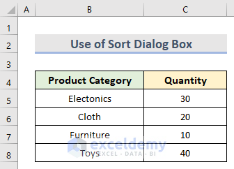
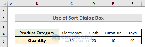
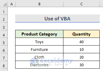
Here, we will learn 4 useful methods to reverse the order of data in Excel. For this, we have used 2 types of datasets in Excel; one is for horizontally and the other one is for vertically reversing the data order that contains the Categories and Quantities of some Products.

Vertical Flip:

Horizontal Flip:

So, without further delay, let’s get started.

1. Reverse Order of Data Using Excel Sort Dialog Box

Here, we will use the Sort dialog box in Excel to reverse the order of data. It is available in the Data tab. The Sort dialog box is the most versatile technique for sorting your data because it allows you to select how you want the data arranged. In this method, we will use this tool both for the column and row order.

1.1 Column Order

The steps to reverse the column order using the Sort dialog box is below.

Steps:

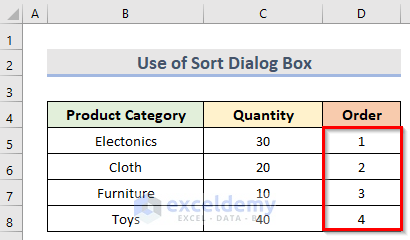
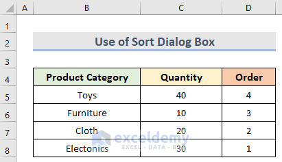
• First, type Order as the column heading in the column adjacent to Quantity.
• Secondly, enter a series of numbers in the Order column (1, 2, 3 & 4) just like the screenshot below.

• Thirdly, select the total dataset (B4:D8).
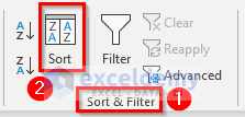
• After that, go to the Data tab.

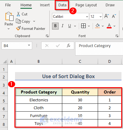
• Then, go to the Sort & Filter group and select the Sort option from there.

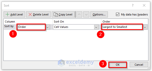
• In turn, the Sort dialog box will pop up.
• Subsequently, select Order from the Sort by dropdown.
• Next, from the Order dropdown, choose Largest to Smallest. See the screenshot below.
• Finally, click OK to reverse the column order.

• In this way, the preceding steps would sort the data based on the values of the Order columns, reversing the order of the names in the data.

Read More: How to Reverse Column Order in Excel

1.2 Row Order

We can also reverse the row order by following the similar process in the above method. Using the Sort left to right feature from the Sort dialog box, we can easily sort the data horizontally. Let’s see the steps to reverse data horizontally of the dataset (B4:F6) below.

Steps:

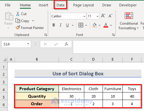
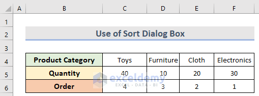
• In the beginning, enter Order as the row’s heading in the row below.
• Then, enter a series of numbers (1, 2, 3 & 4) in the Order row.
• Next, in addition to the Order row, select the whole dataset.
• After that, go to the Data tab.

• Now, from the Sort & Filter group, click on the Sort option.

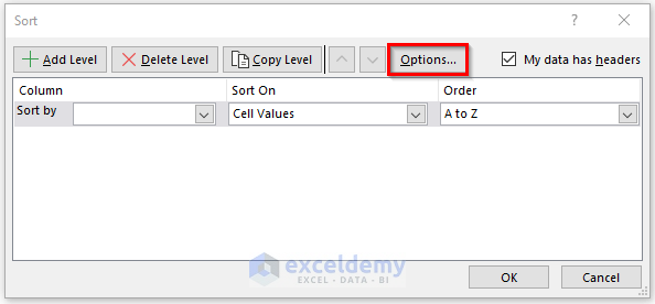
• In turn, the Sort dialog box will appear.
• Afterward, click on Options in the Sort dialog box.

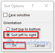
• Therefore, the Sort Options dialog box will open up and you need to click on the Sort left to right.
• Click OK.

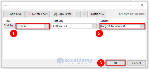
• Again, go to the Sort dialog box and select Row 6 from the Sort by dropdown (the row that contains the Order of your dataset).
• Consequently, select Largest to Smallest from the Order dropdown.
• Click the OK button.

• Thus, the preceding steps would result in a horizontal flip of the entire dataset (B4:F6).

2. Use Excel Data Tab to Reverse Order of a Table

In this method, we will learn to use the Data tab in Excel to reverse the order of the table (B4:D8) below. Here, we need to add the Order column again like the previous methods. Let’s see the steps below.

Steps:

• In the first place, select the values (D5:D8) under the Order column.
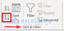
• Then, go to the Data tab.

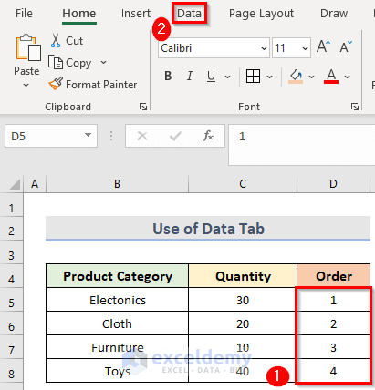
• Now, click on the option (see the screenshot below) from the Sort & Filter group.

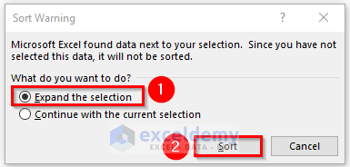
• Eventually, the Sort Warning dialog box will appear.
• At this moment, select Expand the selection from the dialog box.
• Afterward, click OK.

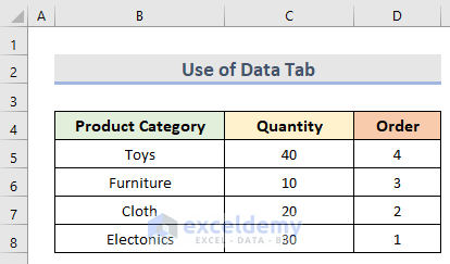
• In this way, we can reverse the data order of an entire table. See the final output in the picture below.

3. Data Order Reversing with Excel Functions

In this method, we will use the SORTBY function and the INDEX function in Excel to reverse the order of data.

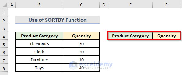
3.1 SORTBY Function

Based on the values of a related range or array, the SORTBY function sorts the contents of a range or array. In this method, we will use the SORTBY function to reverse the data order of the below dataset (B4:C8) in Excel. Let’s see the steps below to do so.

Steps:

• First, copy the table headers (Product Category & Quantity) and paste them into the location (cells E4 & F4) where you want the reversed table.

• Therefore, go to the cell (E5) of the left-most header.
• Then, to reverse the data order type the following formula in the cell:

• In the end, press the Enter key and thus you will get the final result like the screenshot below.

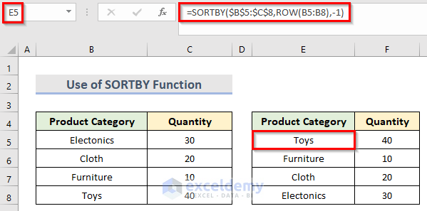
Here, the range $B$5:$C$8 indicates the contents of the whole dataset. The $ sign is for locking the range.

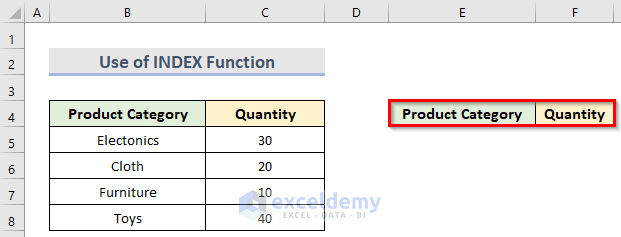
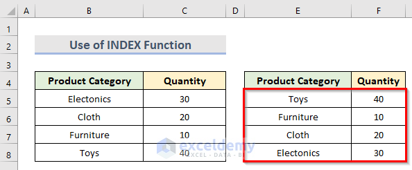
3.2 INDEX Function

We usually use the INDEX function in Excel to return a value from a table or range, or a reference to a value. Here, we will use this function to reverse the order of data in the table (B4:C8) below. The steps to do so are below.

Steps:

• First, place the column headers in the specific location just like the previous method.

• Eventually, to reverse the order of data, type the following formula in cell E5:

• After pressing Enter, you will get the last content of the column.

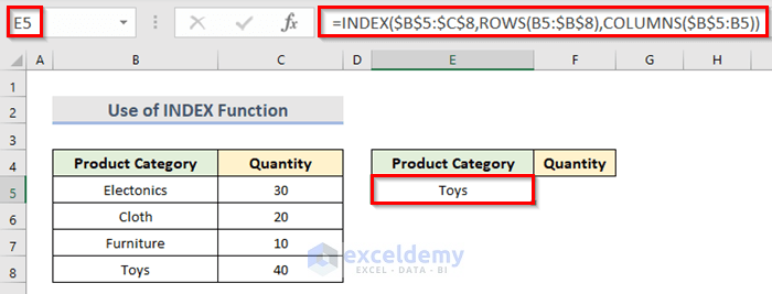
• Lastly, drag the fill handle both right & down to get the entire reversed table (E5:F8).

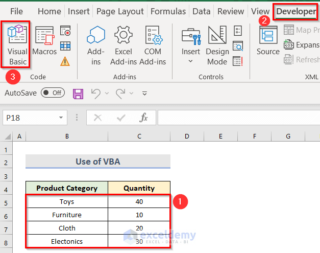
4. Apply VBA in Excel to Flip Data

In our earlier methods, we either utilized an Excel command or a function to reverse data. In our fourth method, we will now use the VBA code in Excel to reverse data both vertically and horizontally.

4.1 Vertical Order

First, we are going to utilize a VBA code in Excel to flip data vertically. However, to achieve the desired outcome, we must enter the proper command and sequence into the code. To gain a clear idea, follow the steps below.

Steps:

• To begin with, choose the B5:C8 data range.
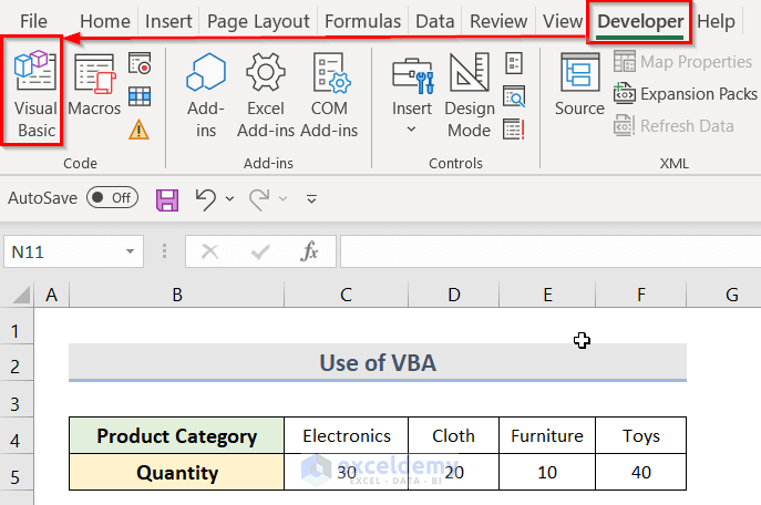
• Eventually, go to the Developer tab and select Visual Basic from the Code group.

• As a consequence, the Microsoft Visual Basic for Applications window will open.
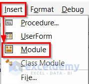
• Next, go to the Insert tab and click on Module.

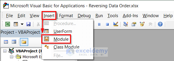
• Hence a Code window will appear.
• You need to insert the VBA code below in the Code window.  Make sure to keep the cursor in the module before clicking the play button.

Sub Reverse_Vertical_Order()
Dim Initial_Row As Variant
Dim Last_Row As Variant
Dim First_Num As Integer
Dim Final_Num As Integer
Application.ScreenUpdating = False
First_Num = 1
Final_Num = Selection.Rows.Count
Do While First_Num < Final_Num
Initial_Row = Selection.Rows(First_Num)
Last_Row = Selection.Rows(Final_Num)
Selection.Rows(Final_Num) = Initial_Row
Selection.Rows(First_Num) = Last_Row
First_Num = First_Num + 1
Final_Num = Final_Num - 1
Loop
Application.ScreenUpdating = True
End Sub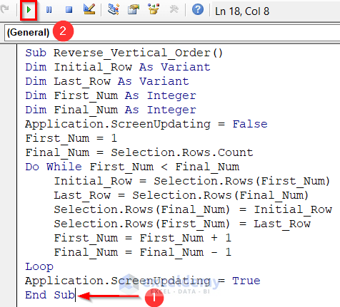

• In this way, we can reverse the order of data in the table successfully.

Read More: How to Reverse Order of Columns Vertically in Excel

4.2 Horizontal Order

Our final step will be to reverse data using another VBA code. However, we will now horizontally invert the data. To do so, follow the steps below.

Steps:

• First, go to the Developer tab and select Visual Basic.

• Second, select the Module from the Insert dropdown.

• Now enter the following VBA code and click the play button after keeping the cursor in the module.

Sub Reverse_Horizontal_Order()
Dim RowRange As Range
Dim RowArray As Variant
Dim Row1 As Integer, Row2 As Integer, Row3 As Integer
On Error Resume Next
RowTitleId = "Reversing Data Horizontally"
Set RowRange = Application.Selection
Set RowRange = Application.InputBox("Cell Range Selection", _
RowTitleId, RowRange.Address, Type:=8)
RowArray = RowRange.Formula
Application.ScreenUpdating = False
Application.Calculation = RowlCalculationManual
For Row1 = 1 To UBound(RowArray, 1)
Row3 = UBound(RowArray, 2)
For Row2 = 1 To UBound(RowArray, 2) / 2
RowArray_Temp = RowArray(Row1, Row2)
RowArray(Row1, Row2) = RowArray(Row1, Row3)
RowArray(Row1, Row3) = RowArray_Temp
Row3 = Row3 - 1
Next
Next
RowRange.Formula = RowArray
Application.ScreenUpdating = True
Application.Calculation = RowlCalculationAutomatic
MsgBox "Done"
End Sub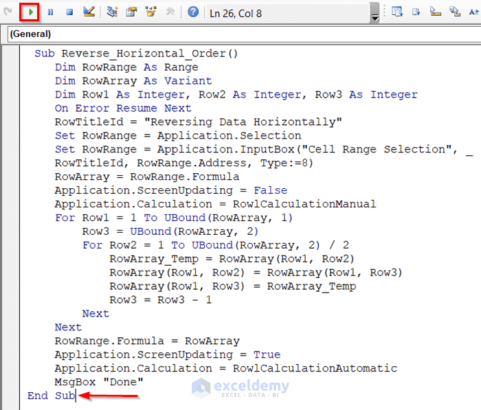

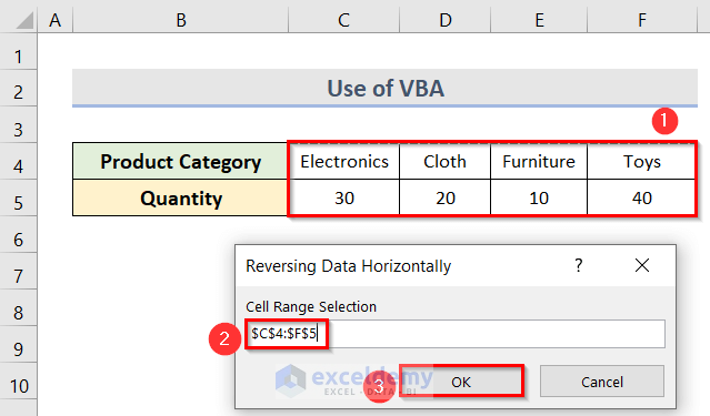
• Consequently, a window named Reversing Data Horizontally will pop up.
• Therefore, you need to select the data range (C4:F5) after keeping the cursor in the Cell Range Selection box.
• Click OK.

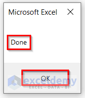
• Thus, the Microsoft Excel window will appear and you need to click OK.

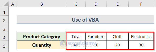
• Finally, after running the code and choosing the cell range, the horizontally arranged data will be flipped.

Things to Remember

• Excel doesn’t have any built-in feature or tool to reverse the order.
• INDEX + ROWS combination will flip the order.
• The Sort option is the best and most straightforward of all the strategies available.
• Knowing VBA macros is necessary to comprehend VBA code.

Download Practice Workbook

Download the practice workbook from here.

Conclusion

I hope the above methods will be helpful for you to reverse the order of data in Excel. Download the practice workbook and give it a try. Let us know your feedback in the comment section.

Related Articles

• How to Reverse Data in Excel Cell
• How to Mirror Data in Excel
• How to Reverse Text to Columns in Excel
• How to Reverse Data in Excel Chart

<< Go Back to Excel Reverse Order | Sort in Excel | Learn Excel