How to Flip Data Horizontally in Excel – 3 Methods

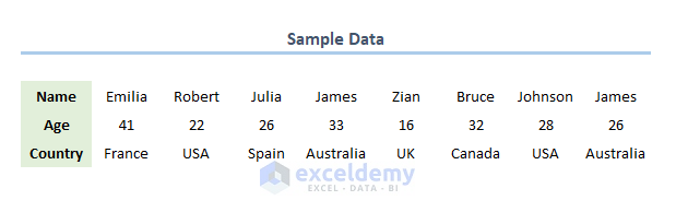
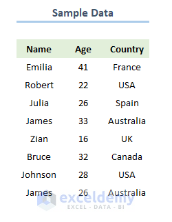
These are the sample datasets.

 

---

Method 1 – Using the Sort Command to Flip Data Horizontally in Excel

 Steps:

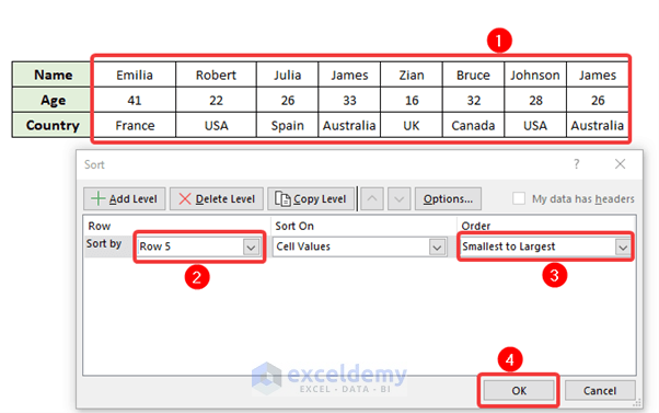
• Select any cell in the dataset. 

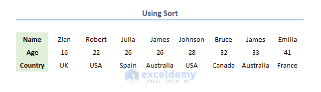
• Click Sort.
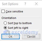
• Choose Options… 

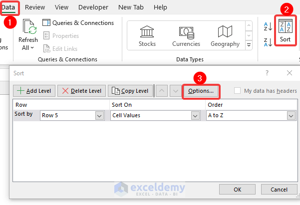
• Check ‘Sort left to right’ and click ‘OK’.

• In Sort by, enter Row 5.
• In Order, choose Smallest to Largest.
• Click OK.

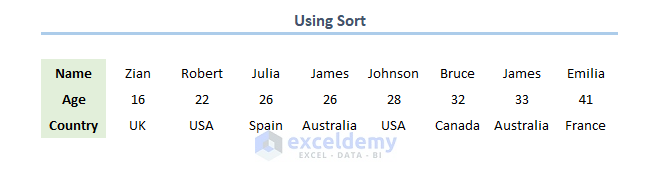
• This is the output.

---

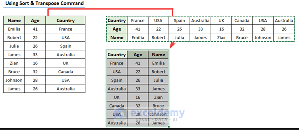
Method 2 – Transpose Twice and Sort with a Helper Column

Steps:

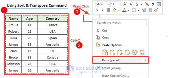
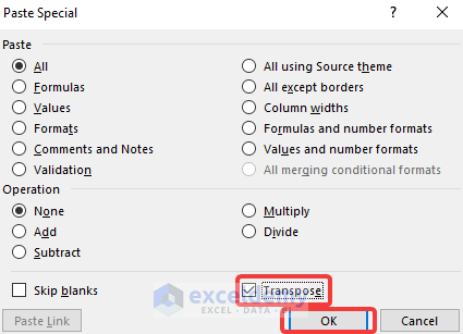
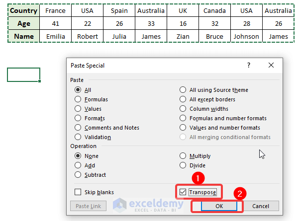
• Select the table and press Ctrl+C to copy >> right-click any cell >> go to Paste Special…

• Add a Helper Column.

• Press Ctrl+C to copy the data table.
• Check Transpose in Paste Special.

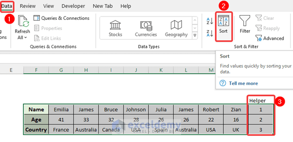
• Select the data to sort and go to Sort in the Data tab.

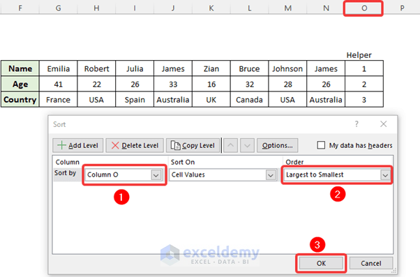
• In Sort By, select COLUMN O.
• In Order, choose Largest to smallest.
• Click OK.

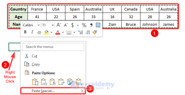
• Press Ctrl+C.
• In Paste Special, check transpose.

This is the output.

Read More: How to Flip Table in Excel

---

Method 3 – Applying a VBA Code to Flip Data Horizontally

Steps:

• Select the table.

• Press Alt+F11.

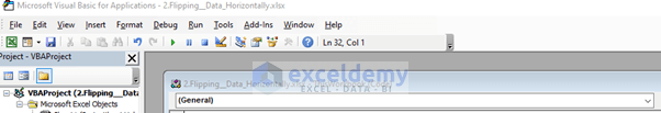
• Enter the VBA code below and press F5.

Sub FlipDataHorizontally()
    Dim xRng As Range
    Dim WrkRng As Range
    Dim ArY As Variant
    Dim i As Integer, j As Integer, k As Integer
    On Error Resume Next
    xTitleId = "Horizontally Flipping Data "
    Set WrkRng = Application.Selection
    Set WrkRng = Application.InputBox("Range", xTitleId, WrkRng.Address, Type:=8)
   ArY = WrkRng.Formula
    Application.ScreenUpdating = False
    Application.Calculation = xlCalculationManual
    For i = 1 To UBound(ArY, 1)
        k = UBound(ArY, 2)
        For j = 1 To UBound(ArY, 2) / 2
            xTemp = ArY(i, j)
           ArY(i, j) = ArY(i, k)
           ArY(i, k) = xTemp
            k = k - 1
        Next
    Next
   WrkRng.Formula = ArY
    Application.ScreenUpdating = True
    Application.Calculation = xlCalculationAutomatic
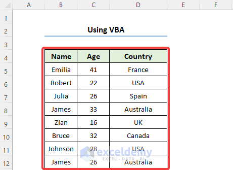
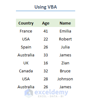
End Sub

This is the output.

---

Download Practice Workbook

Download the practice workbook.

---

Related Articles

• How to Flip Data in Excel Chart
• How to Flip Data Vertically in Excel
• How to Mirror Data in Excel
• How to Reverse Text to Columns in Excel
• How to Reverse Column Order in Excel
• How to Reverse Data in Excel Chart

---

<< Go Back to Excel Reverse Order | Sort in Excel | Learn Excel

Get FREE Advanced Excel Exercises with Solutions!