Download Practice Workbook
The TRANSPOSE Function in Excel
The transpose function converts rows into columns and columns into rows. The basic formula is :
=TRANSPOSE(array)You have to enter the range of cells as an array and press Ctrl+Shift+Enter (older Excel versions) or Enter (Excel 365).
The sample dataset showcases football players’ information.
![]()
Steps:
- Select a range of cells to paste the formula. (re-arrange the orientation. Here, there are 4 columns: the new array will have 4 rows. There are 5 rows: the new array will have 5 columns.
- Enter the following formula in B11.
=TRANSPOSE(B4:E9)
- Press Enter.
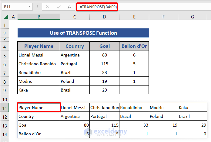
Data is transposed.
- Add borders.
![]()
Example 1 – Conditional Transpose of Data for More Than a Number of Rows
The dataset below contains values in a single column.
![]()
To transpose that column into a single row with the condition: “transpose the column if there are more than 6 rows”.
Steps:
- Select a cell to paste data.
- Enter the formula:
=IF(COUNTA($B$5:$B$11)>6,TRANSPOSE($B$5:$B$11),"")
- Press Enter.
Data will be transposed into a new array.
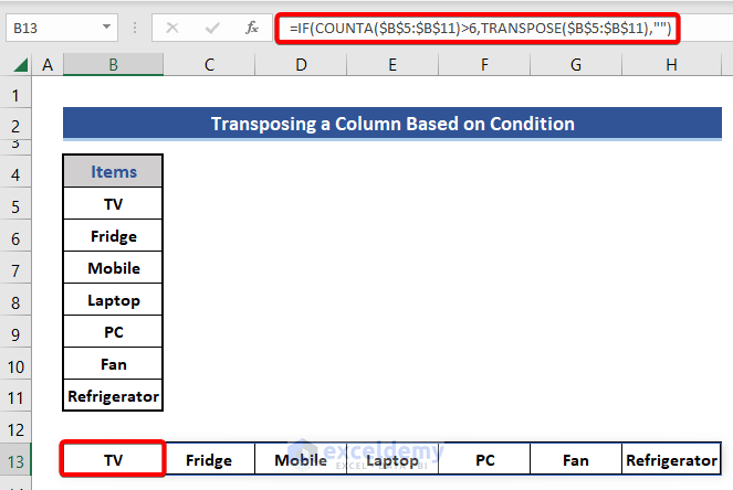
The COUNTA Function counts the number of rows in the column.
You can also use the following formula based on the COUNT function for numeric data:
=IF(COUNT($B$5:$B$11)>6,TRANSPOSE($B$5:$B$11),"")
Read More: How to Convert Single Columns to Rows in Excel with Formulas
Similar Readings
- How to Transpose Duplicate Rows to Columns in Excel (4 Ways)
- Transpose Multiple Columns into One Column in Excel (3 Handy Methods)
- How to Reverse Transpose in Excel (3 Simple Methods)
- Convert Columns to Rows in Excel Using Power Query
- How to Change Vertical Column to Horizontal in Excel
Example 2 – Merge an IF Condition While Transposing Data in Excel
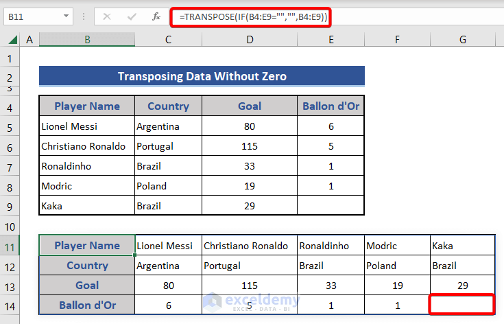
This is the transposed dataset in the section “The Transpose Function in Excel”
![]()
E9 was blank, but in the transposed array the value was set to 0. To avoid this, use conditional transpose:
Steps:
- Select a range of cells to paste data.
- Enter the formula :
=TRANSPOSE(IF(B4:E9="","",B4:E9))
Read More: How to Transpose a Table in Excel (5 Suitable Methods)
Further Readings
- Data clean-up techniques in Excel: Changing vertical data to horizontal data
- How to Swap Rows in Excel (2 Methods)
- How to Transpose Rows to Columns Using Excel VBA (4 Ideal Examples)
- Excel Transpose Formulas Without Changing References (4 Easy Ways)
- How to Transpose Every n Rows to Columns in Excel (2 Easy Methods)
- How to Convert Column to Comma Separated List With Single Quotes


I have a query i have list in column i want to transpose that list in multiple column list is having a blank column so that next transpose set should be in next column if blank cell arises. Very helpfull if you resolve my query.
Hi Akhil,
Unfortunately, there are no direct ways or simple formulas to do that. One way to work around this is to remove the columns as the entirety of them is empty. And then try transposing. Or you can try out VBA to remove the empty columns/rows then try using transpose commands.