Observe the following dataset and the corresponding chart.
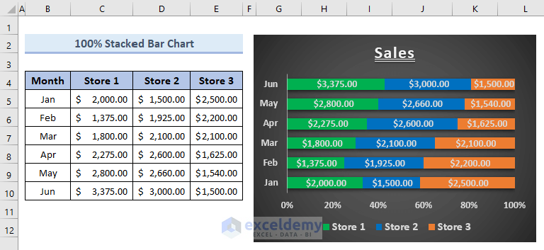
It’s a 100% stacked chart of 3 stores’ sales data.
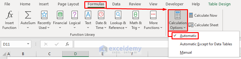
Reminder:
If your Calculation Options (in the Formulas tab, Calculation group) is not set to Automatic, you need to press F9 to update.
Solution 1 – Converting Data into an Excel Table
Steps:
- Select your data and go to the Insert tab.
- Click Table to open the Create Table window.
- Check My table has headers.
- Click OK.

- Add a new column or row and enter the values; Excel will automatically update the chart.
Note:
There should be no blank rows or columns between the new and the last entry.
Solution 2- Setting a Dynamic Formula to Each Data Column
Step 1: Create Defined Names and Set Dynamic Formulas for Each Data Column
- Go to Formulas >> Click Defined Names and choose Define Name.
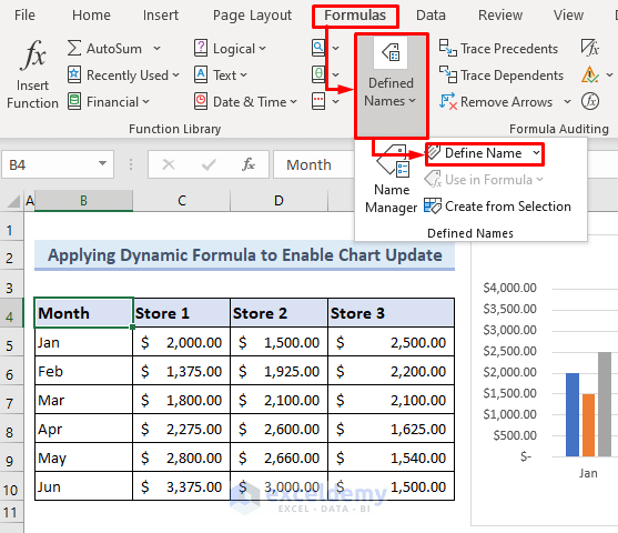
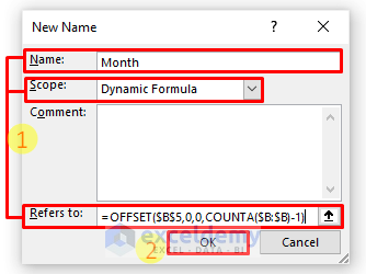
The New Name window will open.
- Enter the first data column header name in the Name: box. Here, Month.
Note:
While defining names, enter an underscore (_) instead of a space.
- In Scope:, select the current worksheet (Dynamic Formula).
- In Refers to:, enter the following formula for the first data column.
=OFFSET($B$5,0,0,COUNTA($B:$B)-1)The OFFSET function refers to the first cell containing data. If your data starts in A2, enter A2 instead of B5. The COUNTA function refers to the whole data column. Change the formula according to your data range.
- Press OK.
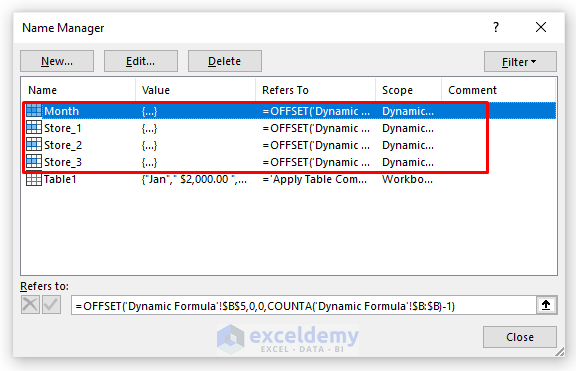
- Repeat the steps for the next 3 data columns. Name them as Store_1, Store_2 & Store_3, and set the following dynamic formulas:
For Store 1:
=OFFSET($C$5,0,0,COUNTA($C:$C)-1)For Store 2:
=OFFSET($D$5,0,0,COUNTA($D:$D)-1)For Store 3:
=OFFSET($E$5,0,0,COUNTA($E:$E)-1)Defined names were created and dynamic formulas set for the data columns.
Step 2: Change Legend Entries and Horizontal Axis Labels with Defined Names
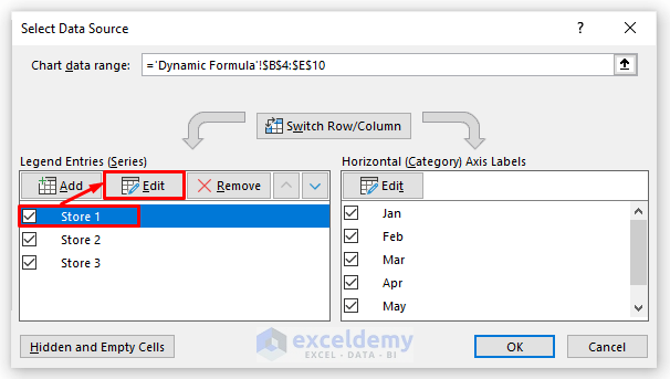
- Click the chart area >> right-click >> choose Select Data.
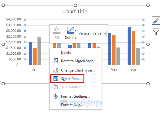
In the Select Data Source window:
- In Legend Entries (Series), select the first entry and click Edit.
- In the Edit Series window, enter ‘Dynamic Formula’!Store_1 in Series values:.
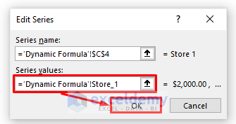
- Click OK.

- Repeat the steps for Store 2 and Store 3.
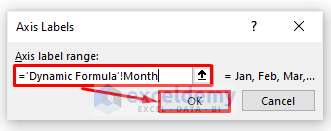
- Go to the Horizontal (Category) Axis Labels and click Edit.
In the new window:
- Replace the cell ranges with the defined name.
- Click OK twice to close the windows.
If you add new data, the Excel chart will update.
Read More: [Solved]: Excel Graph Is Not Showing All Dates
Download the practice workbook here.
<< Go Back to Excel Chart Not Working | Excel Charts | Learn Excel
Get FREE Advanced Excel Exercises with Solutions!
