[Solved]: Excel Graph Is Not Showing All Dates (with Easy Steps)

When you make a graph from worksheet data containing dates, the dates are projected along the horizontal axis of the graph. Excel switches the horizontal axis to a date axis naturally. A date axis can be manually switched from a  horizontal axis. Even if the dates on the worksheet are not in the correct sequence or have different reference units, a date axis exhibits dates chronologically at fixed intervals or based units, such as the number of days, months, or years. This article will demonstrate a step-by-step solution if the Excel graph is not showing all dates.

Download Practice Workbook

You may download the following Excel workbook for better understanding and practice it by yourself.

Step-by-Step Solution If Excel Graph Is Not Showing All Dates

Excel chooses the almost negligible difference between any two time periods in the worksheet data as the basis for the units for the date axis. You can change the unit in Excel from days to months or years if you want to look at how the product performs over a longer time period, like in the case of data for product prices, where the least difference between dates is one day. So, to know the step-by-step solution if the Excel graph is not showing all dates, you can follow the given steps accordingly.

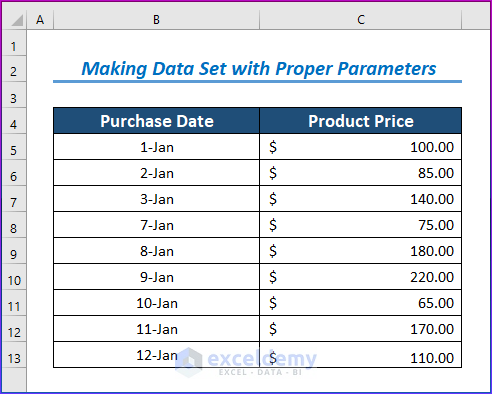
Step 1. Making Data Set with Proper Parameters

In this step, we will create our data set, including some products’ price and their purchase date.

• In order to create a chart, we will first create a data set.

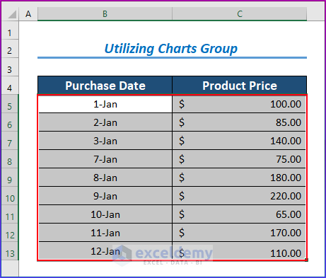
Step 2. Utilizing Charts Group

Excel’s charts group provides a range of chart types. In particular, many charting tools enable users to visualize complex data in straightforward, graphical forms.

• Firstly, select the Product Price and Purchase Date column.

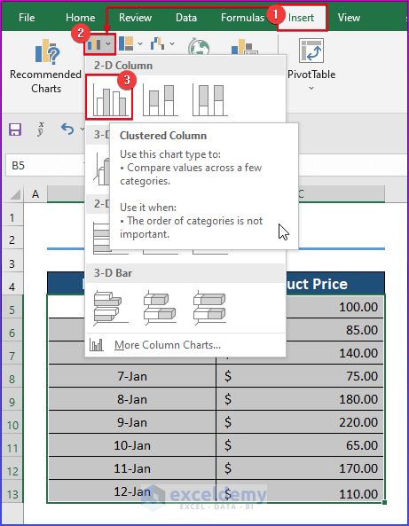
• Firstly, go to the Insert tab after selecting the data range from the given data set.
• Secondly, choose the Insert Column or Bar Chart from the Charts
• Thirdly, select the Clustered Column option from the 2-D Column.

Read More: Selecting Data in Different Columns for an Excel Chart

Step 3. Creating Excel Graph

When comparing precise data groups like frequency, quantity, range, or measurements, bar charts can be helpful. They are also employed to show patterns.

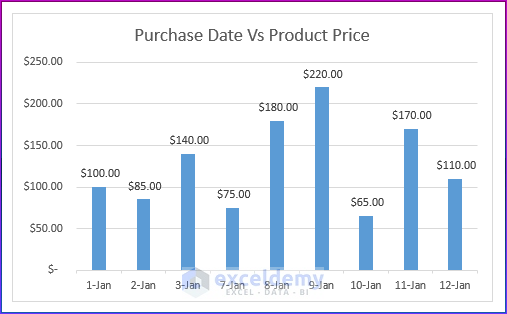
• As a result, you will see the output graph in the below image.
• So, you will see in the data set that some of the dates are missing and the Excel creates some blank space for the missing dates.

Read More: How to Group Data in Excel Chart (2 Suitable Methods)

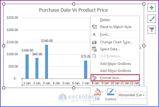
Step 4. Utilizing Format Axis Command

Excel offers date-display options that can close this blank space by utilizing the Format Axis command.

• Firstly, right-click on the X-axis.
• Then, choose the Format Axis command.

• After that, the Format Axis window will open.
• Besides, select the Text Axis option from the Axis options.

Step 5. Showing Final Output

• Finally, you will see the final output in the below image. The results will be comprised of all the dates including.

Read More: How to Show Only Dates with Data in Excel Chart

Conclusion

In this article, we’ve covered step-by-step solutions If the Excel graph is not showing all the dates. We sincerely hope you enjoyed and learned a lot from this article. Additionally, if you want to read more articles on Excel, you may visit our website, ExcelDemy. If you have any questions, comments, or recommendations, kindly leave them in the comment section below.

Related Articles

• How to Get Data Points from a Graph in Excel (2 Easy Ways)
• Excel Chart Disappears When Data Is Hidden (3 Solutions)
• How to Sort Data in Excel Chart (5 Easy Methods)
• Excel Chart by Month and Year (2 Suitable Examples)
• How to Change Date Range in Excel Chart (3 Quick Ways)
• Edit Chart Data in Excel (5 Suitable Examples)
• How to Format Data Series in Excel (with Easy Steps)