Excel Chart Disappears When Data Is Hidden (3 Solutions)

Sometimes for data visualization, you may need to use an Excel chart. But when you hide your data, your chart may disappear. So, if you find the solutions to why an Excel chart disappears when data is hidden. Then you have come to the right place.

In this article, I will explain the solutions to why an Excel chart disappears when data is hidden. Additionally, for conducting the session, I’m going to use Microsoft 365 version.

Excel Chart Disappears When Data Is Hidden: 3 Possible Solutions

Here, I will describe 3 suitable solutions to why an Excel chart disappears when data is hidden. In addition, for your better understanding, I’m going to use a sample dataset. Which contains 3 columns. They are Product, Sales, and Profit. The dataset along with the chart is given below.

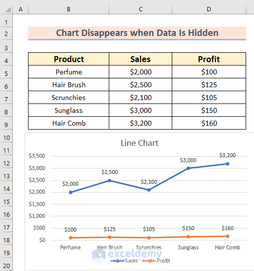
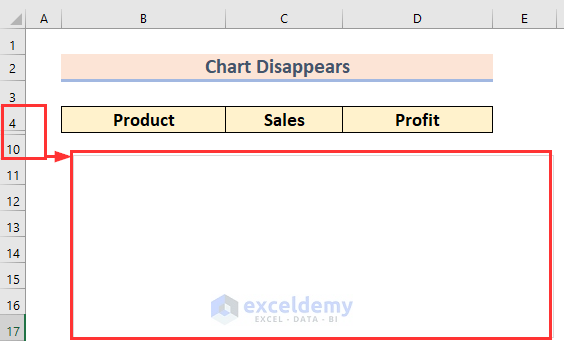
Here, you can see that when I have hidden rows 5 to 9. Then the Excel chart disappears. Now, I will show the solutions to not disappear from your chart even if you hide the data.

1. Using Chart Tools to Show Chart When Data Is Hidden

Here, I will use the Chart tools as a solution to not disappear the chart in Excel even if you hide the related data.

Solutions:

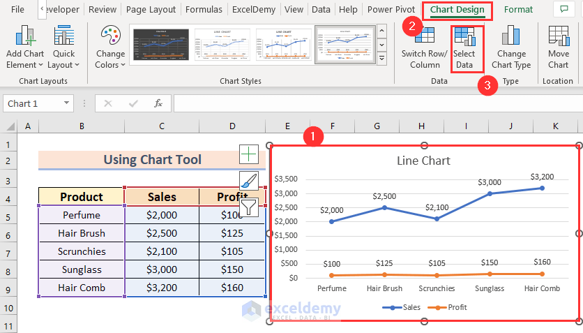
Firstly, select the chart.

As a result, you will see two new contextual tabs in the custom ribbon.

Secondly, from the Chart Design tab >> go to the Select Data option.

After that, you will see the following dialog box named Select Data Source.

Now, from the dialog box of Select Data Source, you have to choose the Hidden and Empty Cells option.

Subsequently, you will see another dialog box named Hidden and Empty Cell Settings.

Then, tick the mark on Show data in hidden rows and columns.
After that, press OK.

Again, the previous dialog box named Select Data Source will appear.

After this, press OK on the Select Data Source box.

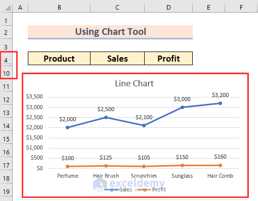
Finally, you will see that I have hidden rows 5 to 9 but still, the Excel chart is visible.

2. Use of Context Menu Bar to Keep Chart Visible

Now, I will use the Context Menu Bar for opening the Select Data feature as a solution to not disappear the chart in Excel even if you hide the related data.

Solutions:

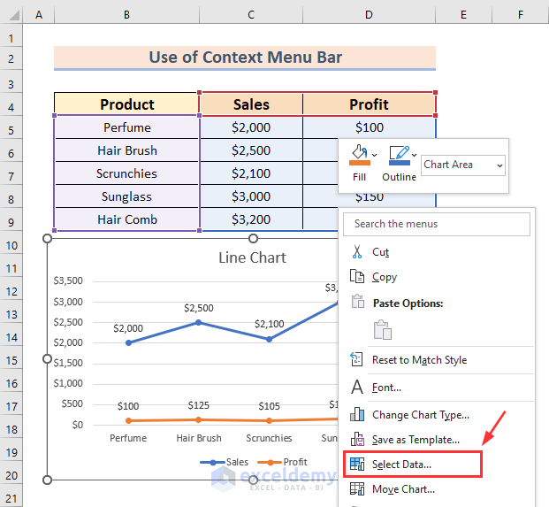
Firstly, right-click on the chart.
Secondly, from the Context Menu Bar >> choose the Select Data option.

After that, you will see the following dialog box named Select Data Source.

Now, from the dialog box of Select Data Source, you have to choose the Hidden and Empty Cells option.
Then, follow the steps of method-1.

Lastly, you will see that if I hide rows 5 to 9 but still the Excel chart will be visible.

3. Applying VBA to Show Chart When Data Is Hidden

Here, you can employ the VBA code as a solution to not disappear the chart in Excel even if you hide the related data. Furthermore, I will explain two different VBA codes to keep the Excel chart visible.

3.1. Always Appearing Excel Chart

The first code is for always appearing in the Excel chart even when you hide the data. Now, follow the steps given below.

Steps:

Firstly, you need to open your worksheet. Here, you must save the Excel file as an Excel Macro-Enabled Workbook (*xlsm).
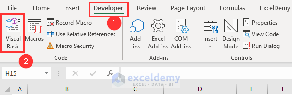
Secondly, you have to choose the Developer tab >> then select Visual Basic.

At this time, from the Insert tab >> you have to select Module.

After that, write down the Code given below in Module1.

Sub chart_appearing_when_data_hidden()
Dim my_chart As Chart
Set my_chart = ActiveChart
On Error Resume Next
my_chart.PlotVisibleOnly = Not my_chart.PlotVisibleOnly
On Error GoTo 0
End Sub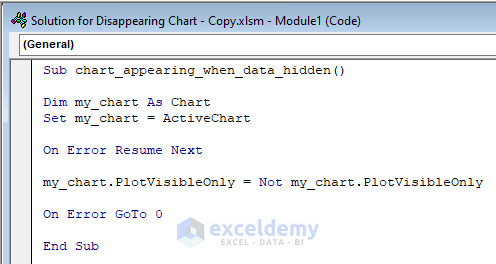

Code Breakdown

Here, I have created a Sub Procedure named chart_appearing_when_data_hidden.
Next, I declare a variable my_chart as Chart.
After that, I used the property PlotVisibleOnly to keep the chart always visible.

Then, Save the code then go back to the Excel File.
Then, from the Developer tab >> select Macros.

At this time, select Macro (chart_appearing_when_data_hidden) and click on Run.

Lastly, you will see that if you hide rows 5 to 9 then still the Excel chart will be visible.

3.2. Keep Visible Excel Chart with Mouse Click

The 2nd code is for keeping the Excel chart visible even when you scroll the data. Now, follow the steps given below.

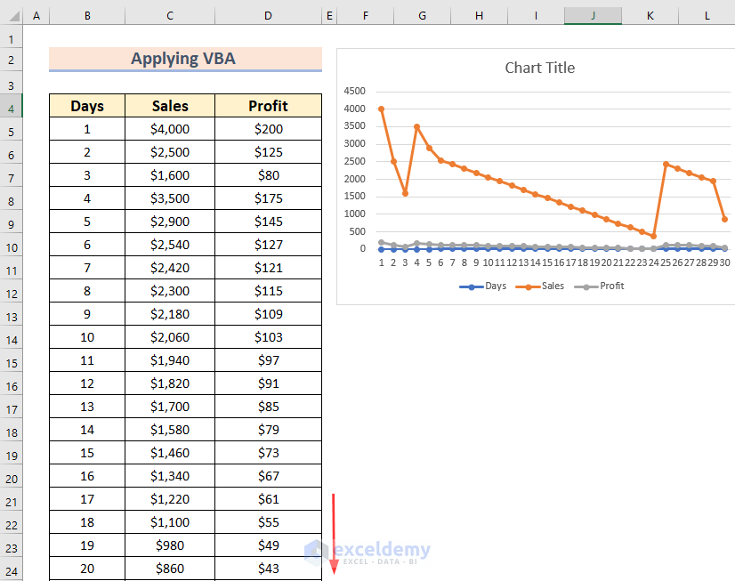
Furthermore, for this method, I’m going to use the following dataset which contains sales recordings for 30 days of a company.

Now, right-click on the worksheet where the data is. Here, I have right-clicked on the worksheet named VBA.
Then, choose View Code.

Then, write the following code.

Private Sub Worksheet_SelectionChange(ByVal Target As Range)
 Dim my_variable As Double
    Application.ScreenUpdating = False
    my_variable = ActiveWindow.ScrollRow * ActiveCell.RowHeight
    ActiveSheet.ChartObjects("Chart 1").Activate
    ActiveSheet.Shapes("Chart 1").Top = my_variable
    ActiveWindow.Visible = False
    Application.ScreenUpdating = True
End Sub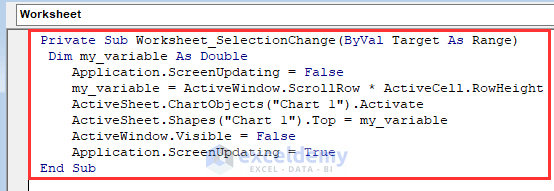

Code Breakdown

Here, I have created a Private Sub Procedure where I’ve selected the event SelectionChange. So that whenever I select any cell the Chart will move along with the selection.
Next, I declare a variable my_variable as Double.
After that, I used some properties to keep the chart always visible.

Furthermore, in the code, Chart 1 is the name of the chart. So, you must write the chart view name of your chart inside the code.

Then, Save the code then go back to the Excel File.
Now, if you click any cell you will see that the chart will be visible there.

How to Resolve the Issue When Charts Are Not Displaying in Excel

Sometimes, you may face another problem like inserting a chart but that chart is not displaying in Excel. In this section, I will demonstrate why an Excel chart is not working.

Basically, if Excel stores the cell’s value as Text format rather than Number format then you may face this problem.

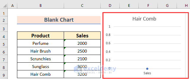
Moreover, I have attached an example of it. Here, if you notice then you will see that the values of the Sales column are stored in Text format.

Now, let’s talk about the solution.

Solution:

Firstly, select the cells C5:C9.
Secondly, from the Dropdown arrow under the Number format >> choose Number.

Then, remove the Apostrophe symbol.

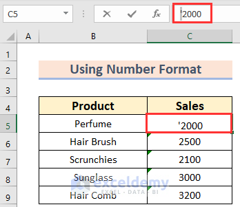
Finally, you have converted the C5 cell value to a Number.

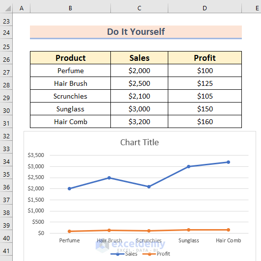
Similarly, convert all the cell values into Numbers.

Lastly, you will see the chart. Here, I have used the Currency sign. This is not mandatory.

💬 Things to Remember

Actually, the easiest and most useful way is to keep the Show data in hidden rows and columns option On.
Furthermore, for hidden cells use 1st code.
Moreover, to keep the chart visible on the worksheet while scrolling data use 2nd code.

Practice Section

Now, you can practice the explained method by yourself.

Download Practice Workbook

You can download the practice workbook from here:

Solution for Disappearing Chart.xlsm

Conclusion

I hope you found this article helpful. Here, I have explained 3 solutions as an Excel chart disappears when data is hidden. Please, drop comments, suggestions, or queries if you have any in the comment section below.

<< Go Back to Excel Chart Not Working | Excel Charts | Learn Excel

Get FREE Advanced Excel Exercises with Solutions!