What Is the x-Intercept?
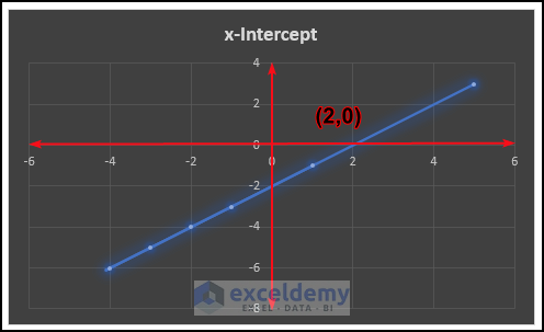
The x-intercept is the x-ordinate of a point on a straight line, where the line intersects the X-axis. If a straight line intersects the X-axis at (2,0), the x-intercept will be 2.
How to Find the X Intercept for Linear Data in Excel
Consider a linear equation (y = 3x – 7). To find the value of X when y = 0:
- Select C12 >> use the following formula >> press Enter.
=INTERCEPT(B6:B10,C6:C10)- Plot a Scatter with Smooth Lines and Markers chart.
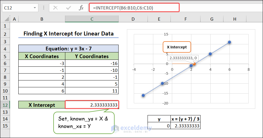
- The INTERCEPT function finds the point at which a line intersects the y-axis. It uses known x-values and known y-values.
- The INTERCEPT function considers the intersection at the y-axis, which means it calculates the y-intercept.
- When you calculate the x-intercept with the INTERCEPT function, your y-values will be INTERCEPT x values and your x-values will be INTERCEPT y-values.
How to Find the x-Intercept in Excel – 5 Methods
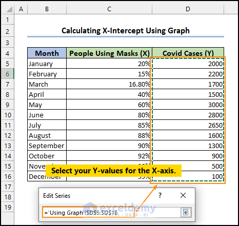
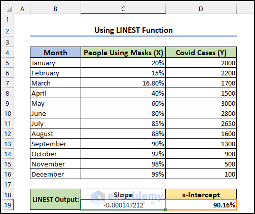
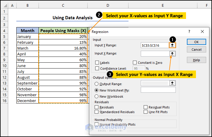
The dataset showcases monthly Covid cases (set as Y-values) and monthly use of masks (set as X-values).
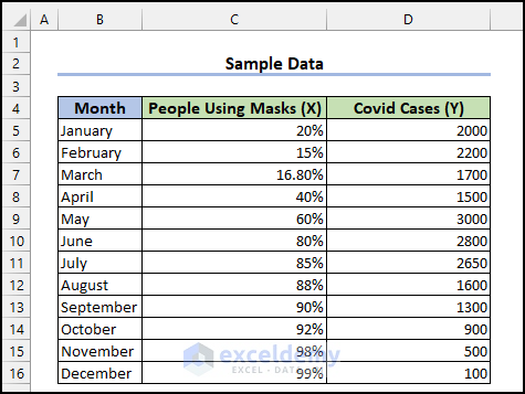
You want to know what is the percentage of people using masks when the number of covid cases becomes zero.
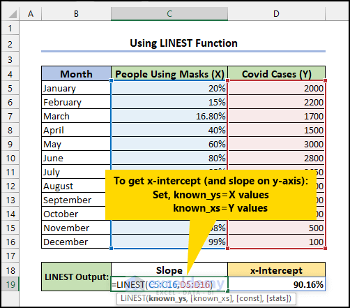
Method 1 – Using the INTERCEPT Function to Find the x-Intercept
Steps:
- Use the following formula in C18 to find the x-intercept.
=INTERCEPT(C5:C16,D5:D16)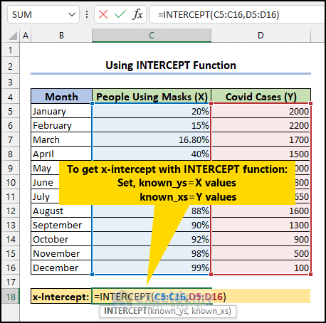
Your x-values=C5:C16 ⇒ y-values in the formula.
Your y-values=D5:D16 ⇒ x-values in the formula.
The x-intercept = 90.16% (after applying the percentage format).
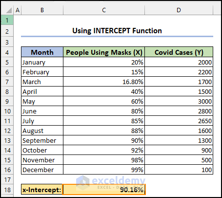
Interpretation of the x-Intercept:
- The y value (covid cases) is set to zero.
- When the use of masks is 90.16%, covid cases will be zero.
- Or, when the covid cases tend to zero, the use of masks is still 90.16%.
Method 2 – Using the FORECAST.LINEAR Function to Find the X-Intercept
Steps:
- Select D19 >> enter the following formula >> click OK.
=FORECAST.LINEAR(D18,C5:C16,D5:D16)
When calculating X Intercept using the FORECAST.LINEAR function, you must switch between the known_ys and know_xs values: People Using Masks (X) as known_ys and Covid Cases (Y) as know_xs.
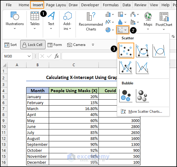
Method 3 – Using the Trendline Equation Feature of Excel Graphs
Steps:
- Go to the Insert tab and click Scatter.
- Select the first icon.
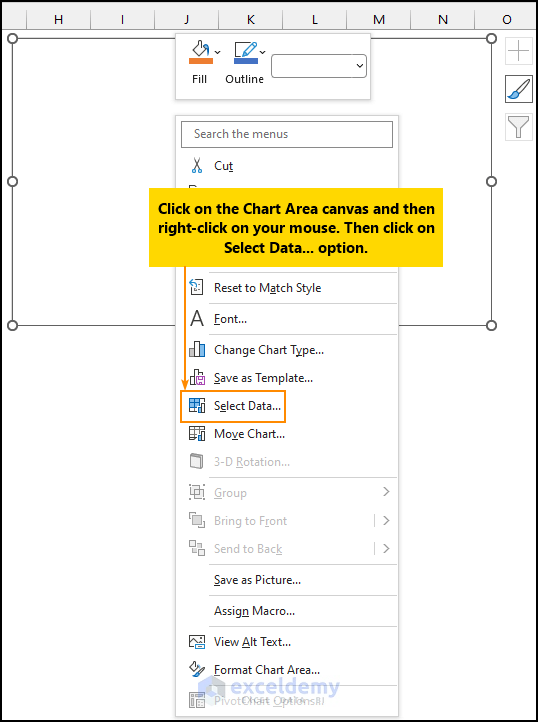
A blank canvas will be displayed.
- Click the Chart Area canvas and right-click.
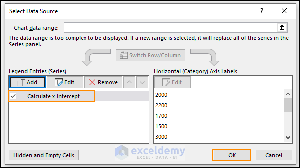
- Click Select Data… option.
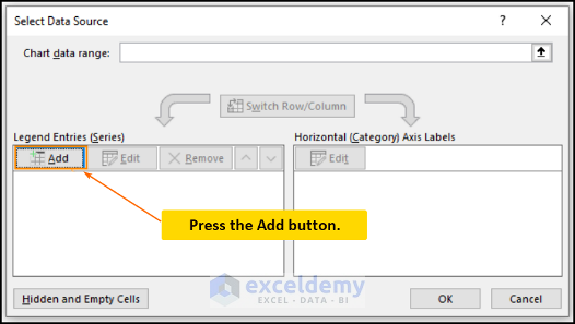
- In the Select Data Source window, click Add.
- In Edit Series, name the series (Calculate x-Intercept).
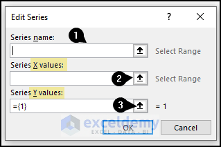
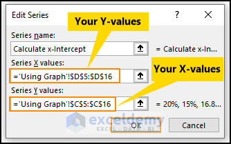
- Choose the X values. (Excel’s X values are equivalent to Y values here.)
- Choose the Y values.
- Click OK.
- The Calculate x-Intercept series is displayed in the Select Data Source window and automatically selected.
- Click OK.
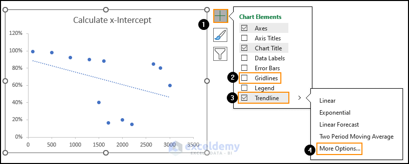
- Click the Chart Elements button (the + sign in the image below).
- Uncheck Gridlines.
- Select Trendline and click the angle icon (〉).
- Select More Options.
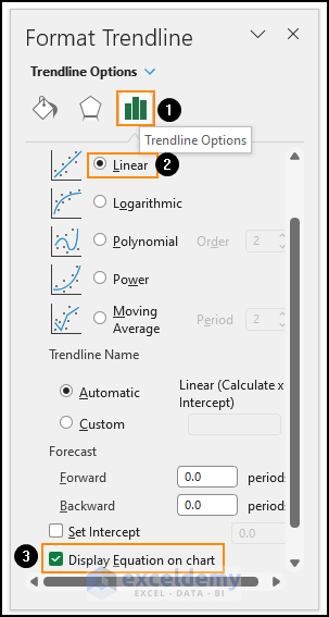
- In Format Trendline, click the 3rd icon (Trendline Options).
- Select Linear.
- Check ‘Display Equation on the chart’.
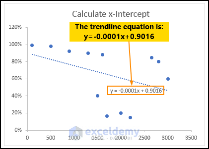
- Go back to the graph.
An equation is displayed in the chart area:
This is the output: the x-intercept is 0.9016 (90.16%, when formatted as a percentage).
Read More: How to Set Intercept Trendline in Excel
Method 4 – Using the LINEST Function to Find the x-Intercept
Steps:
- Use the formula in C19:
=LINEST(C5:C16,D5:D16)- Press ENTER.
The intercept is displayed in C20 (and the slope in C19).
Read More: How to Find Intercept of Two Lines in Excel
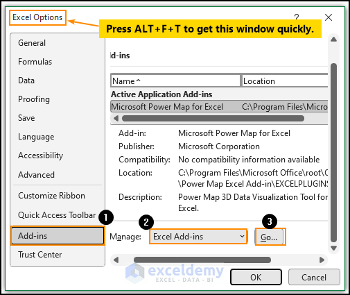
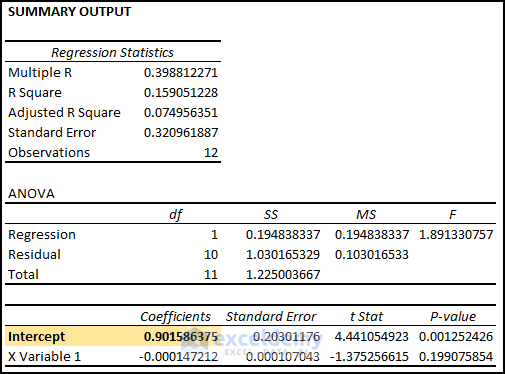
Method 5 – Using the Data Analysis ToolPak
Steps:
- To enable the Data Analysis ToolPak, press ALT+F+T and go to the Excel Options window.
- Select Add-ins and choose Excel Add-ins in Manage.
- Click Go.
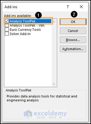
- In Add-ins, check Analysis ToolPak.
- Click OK.
- The feature is displayed on the ribbon.
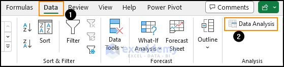
- Go to the Data tab and click Data Analysis in Analysis.
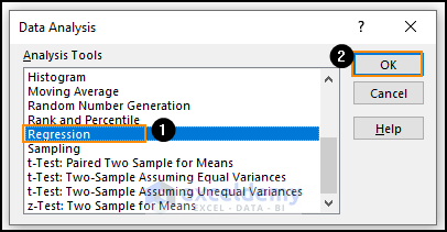
- In Data Analysis, select Regression and click OK.
- In the Regression window, Enter the Input Y Range (remember you have to select your X-values here).
- Enter the Input X Range.
- Click OK.
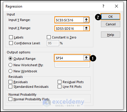
- In the Regression window, select a location to place the Output Range (here, F4).
- Click OK.
The regression summary will be generated by ToolPak. You will see the x-intercept and other statistic data.
Read More: How to Find Y Intercept in Excel
Download Practice Workbook
Download the following workbook.
<< Go Back to Excel INTERCEPT Function | Excel Functions | Learn Excel
Get FREE Advanced Excel Exercises with Solutions!

Hey, these 4 methods to determine an x-intercept for a data set are wrong. You have to determine the x incept for a given line by solving the equation of a line for x and setting y=0. None of these methods provide and even close to accurate value for a data sets linear regression line’s x-intercept. READER BEWARE.
Hello Dr Timber
I went through this article and did not find any technical issues. In my view, you should reconsider what you have said.
This article is about finding an X intercept. To demonstrate this point, this context considers a practical dataset where the percentage of people still using masks is calculated when the number of Covid Cases becomes Zero. I think you expected the calculation to find X Intercept for Y = 0. That’s what is calculated in those methods. When the writer introduced us to the dataset, it was explicitly mentioned.
Anyway, I am introducing another method that may overcome your confusion. I have calculated the percentage of people who still use masks when the number of Covid Cases becomes Zero. I am using FORECAST.LINEAR Function to predict the percentage. And I get the same result shown in this article.
Excel Formula:
The data considered in this article is not Linear. That’s why you get confused. However, these methods must be able to find an X intercept for any Linear data.
Stay safe. And good luck!
Regards
Lutfor Rahman Shimanto