How to Find the Intercept of Two Lines in Excel – 3 Methods

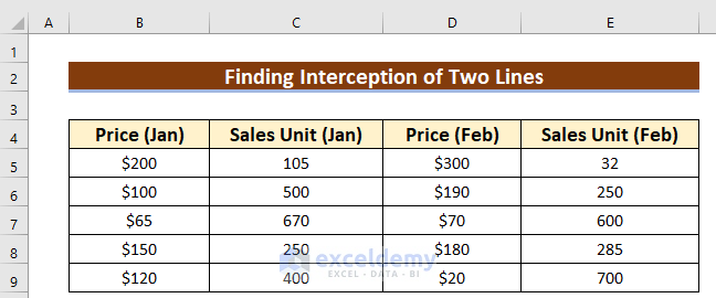
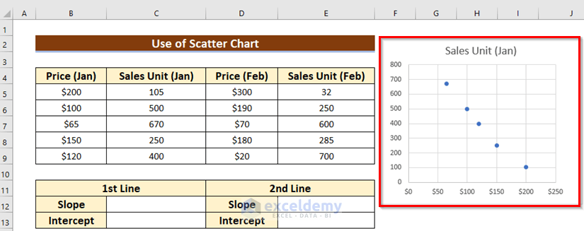
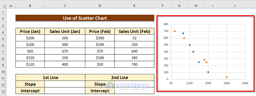
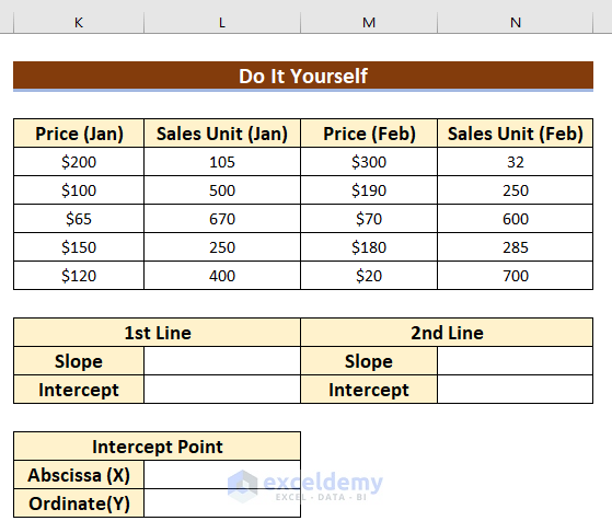
The sample dataset showcases prices and sales data in January and February.

Method 1 – Combining the SLOPE & INTERCEPT Functions to Find a Common Point in Excel

Steps:

• Select a new cell: C12, to keep the slope of the 1st line.
• Use the formula below in C12.

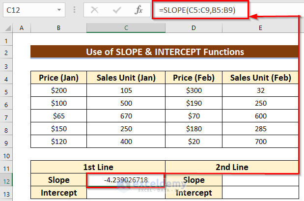
The SLOPE function returns the slope of the equation. C5:C9 is the y range and B5:B9 is the x range.

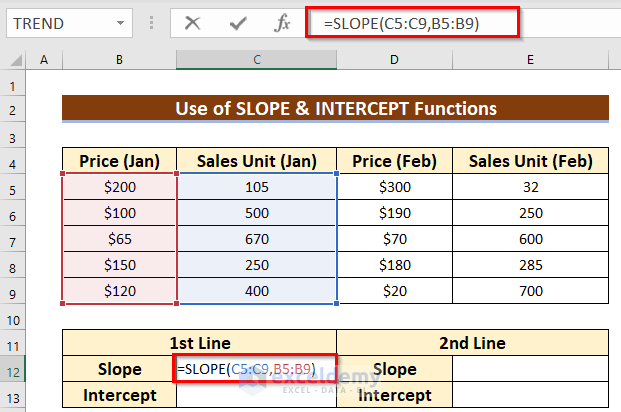
• Press ENTER.

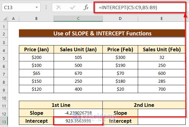
• Enter the formula in C13 to find the intercept of the 1st line.

The INTERCEPT function returns the intercept of the equation using a regression analysis. C5:C9 is the y range and B5:B9 is the x range.

• Press ENTER to see the intercept of the 1st line.

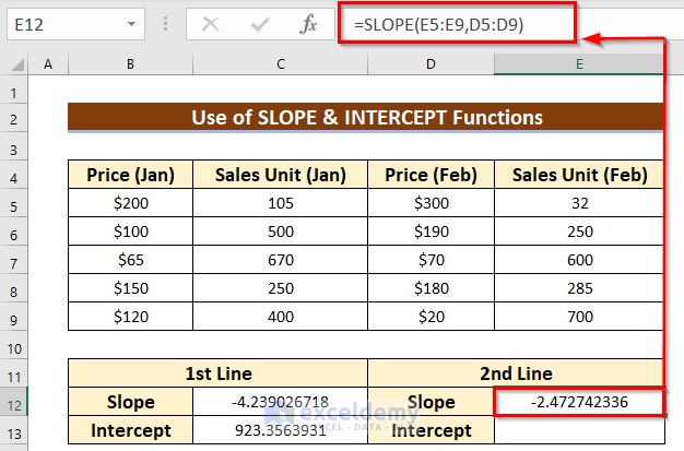
• Enter the formula below in E12 to find the slope of the 2nd line.

The SLOPE function returns the slope of the equation. E5:E9 is the y range and D5:D9 is the x range.

• Press ENTER to see the slope of the 2nd line.

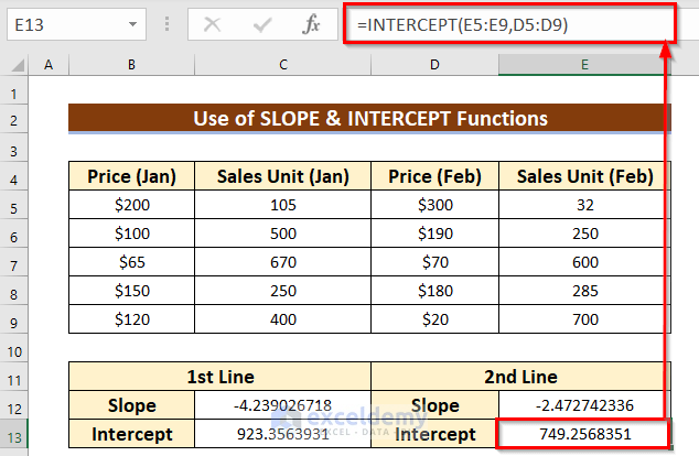
• Enter the formula in E13 to find the intercept of the 2nd line.

The INTERCEPT function returns the intercept of the equation using a regression analysis. E5:E9 is the y range and D5:D9 is the x range.

• Press ENTER to see the intercept of the 2nd line.

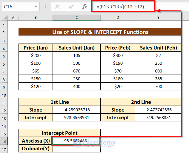
Find the coordinate of the intercept point.

• In C16, use the following formula.

• Press ENTER, and you will get the abscissa (X) of that point.

• Use the formula below in C17.

• Press ENTER, and you will get the ordinate (Y) of that point.

Read More: How to Find x-Intercept in Excel

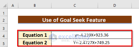
Method 2 – Utilize the Goal Seek Feature to Find a Common Point of Two Lines

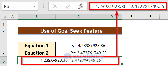
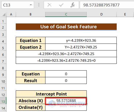
You have the following two equations and want to know their intercept point.

Steps:

• Enter the equations in B6 using the Apostrophe (‘). Here, B6:D6 were merged. The Apostrophe (‘) denotes this is a text.

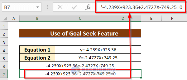
• Move the right-hand side to the left-hand side, using the equation law.

• Use the C13 cell reference instead of X in the above equation and keep it in C9.

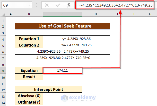
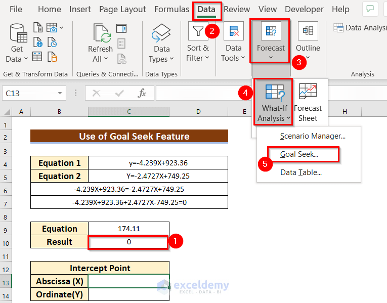
• Enter “0” in C10 (the equation must be equal to zero).
• In the Data tab >> go to Forecast >> What-If Analysis >>Goal Seek.

In the Goal Seek dialog box:

• Use the C9 cell reference in Set cell.
• Enter 0 in To value.
• Select C13 in By changing cell.
• Click OK.

In Goal Seek Status:

• Click OK.

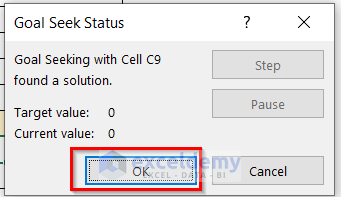
You will see the abscissa (X) of that intercept point.

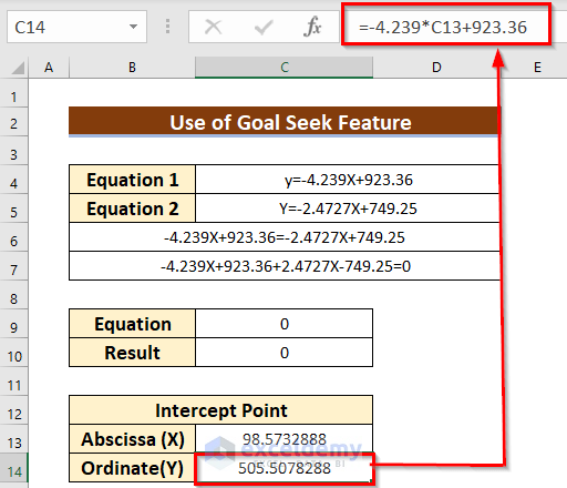
• Use the following formula in C17.

C13 cell value (X) is used in the 1st equation to find the Y value.

• Press ENTER to see the ordinate (Y) of that point.

Method 3 – Use the Excel Scatter Chart to Find the Intercept of Two Lines

Step 1: Find Linear Equations for Two Lines in Excel

• Select the data of the 1st line. Here, B4:C9.
• Go to the Insert tab.
• In Charts, go to Insert Scatter (X, Y) or Bubble Chart >> choose Scatter.

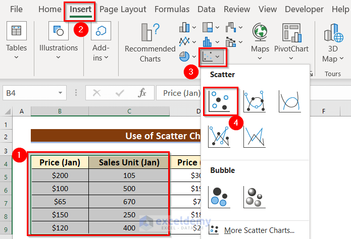
• You will see the following scatter points of the 1st line.

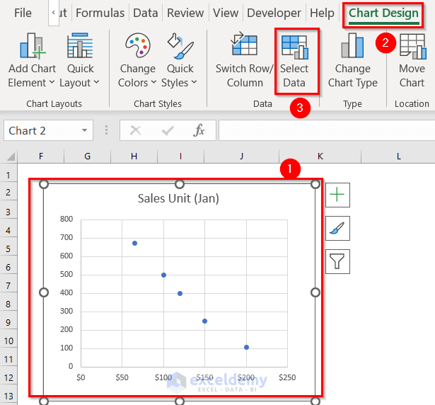
• Select the Chart.
• In Chart Design >> go to Select Data in Data.

The Chart Design tab will only displayed o the ribbon if the chart is selected. You can display it by Right-Clicking the Chart and using the Context Menu Bar.

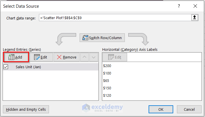
You will see the Select Data Source dialog box.

• Choose Add.

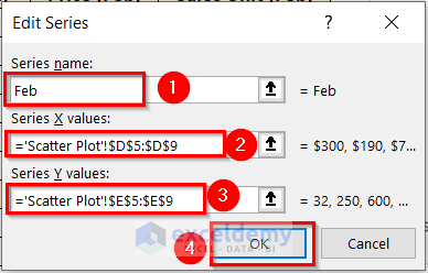
In Edit Series:

• Enter or select the Series name. Here, Feb.
• Enter the Series X values. Here, D5:D9.
• Enter the Series Y values. Here, E5:E9.
• Click OK.

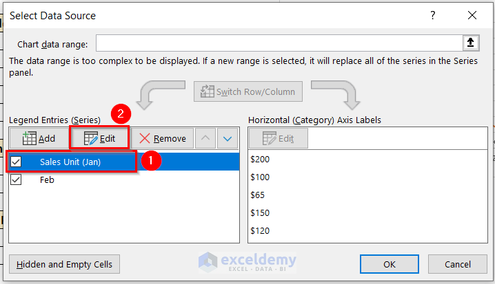
In Select Data Source:

• Select Sales Unit (Jan) >> choose Edit.

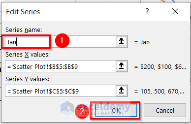
In Edit Series:.

• Enter the Series name. Here,  Jan.
• Click OK.

• Click OK in the Select Data Source box.

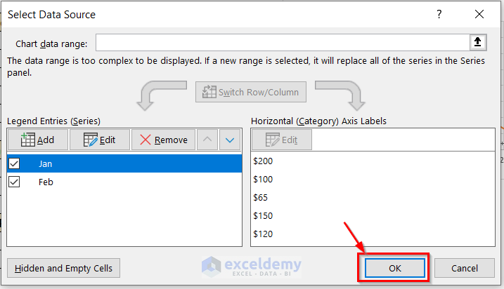
• You will see the points of the 2nd line.

• Click the scatter points of the 1st line.
• Click the Plus icon >> go to Trendline >> choose Linear.

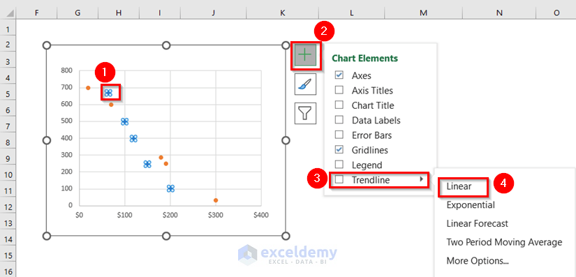
A trendline is added to the 1st line.

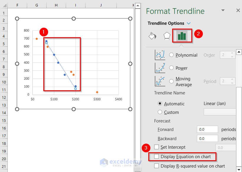
• Double-click that line.

In Format Trendline:

• Select Trendline Options >> check Display Equation on chart.

• In Fill & Line >> change the Dash type to Solid line.

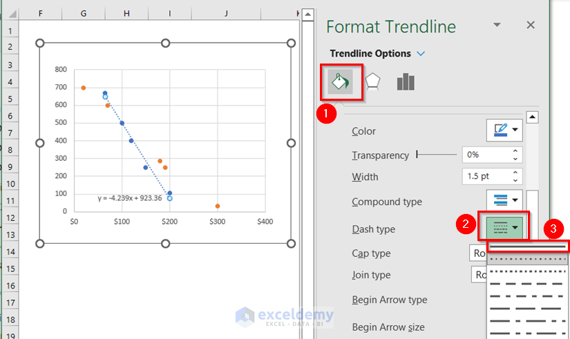
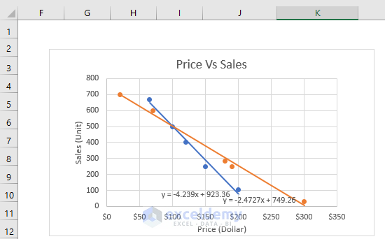
• You will see the equation of the 1st line.

The equation format is Y=mX+c.  m is the slope and c is the intercept.

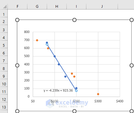
• Find the equation for the 2nd line.

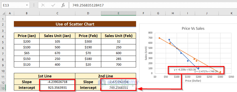
Step 2: Find the Coordinate of the Intercept Point of Two Lines in Excel

• Enter the values of slope and intercept for both lines using the equations.

To find the coordinate of that intercept point:

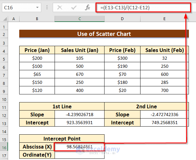
• In C16, use the following formula.

• Press ENTER, and you will see the abscissa (X) of that point.

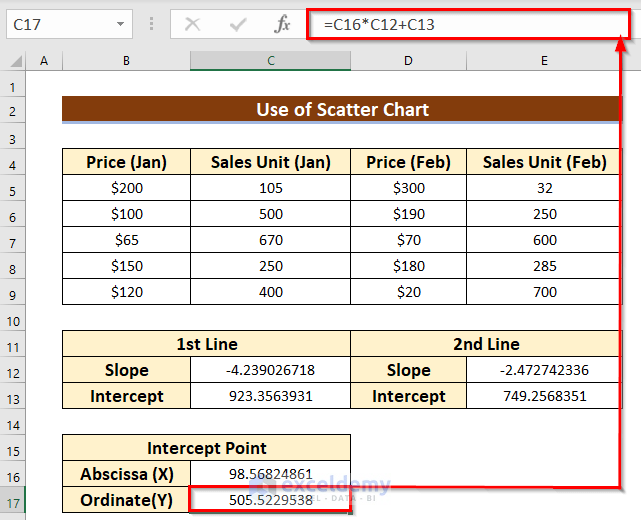
• Use the formula below in C17.

• Press ENTER, and you will see the ordinate (Y) of that point.

Read More: How to Set Intercept Trendline in Excel

Practice Section

Practice here.

Download Practice Workbook

Download the practice sheet.

Related Articles

• How to Find Y Intercept in Excel

<< Go Back to Excel INTERCEPT Function | Excel Functions | Learn Excel