In scientific research, it is required to calculate predicted values. Because in market research or data science, prediction is usually more significant. Therefore, the INTERCEPT function is more important here. The INTERCEPT function in Excel is a built-in function that is categorized as a Statistical Function. Using existing x- and y-values, the INTERCEPT function calculates the location at which a line will intersect the y-axis. By plotting a best-fit regression line through known x- and y-values determines the intercept point.
In this tutorial, we will discuss the INTERCEPT function in Microsoft Excel along with its formula syntax and usage. In addition, we will plot a regression line using the INTERCEPT function to make it visualized.
INTERCEPT Function in Excel: Syntax
Function Objective:
Based on known x and y values, the INTERCEPT function in Excel determines the location where a regression line will intersect the y-axis.
Syntax:
=INTERCEPT(known_y’s, known_x’s)
Arguments Explanation:
| Argument | Required/Optional | Explanation |
|---|---|---|
| Known_y’s | Required | The dependent set of observations or data. |
| Known_x’s | Required | The independent set of observations or data. |
Return Parameter:
The INTERCEPT function gives you a number. It will return the #N/A error if the known y values and known x values arguments have different numbers of items.
Equation
In a regression model, interpreting the intercept isn’t always as simple as it appears. When all X=0, the intercept is the predicted mean value of Y.
So, let’s start with a single predictor, X, in a regression equation.
![]()
If X equals 0 on occasion, the intercept is simply Y’s expected mean value at that point. That’s significant. The intercept has no intrinsic value if X never equals 0. Both of these instances occur frequently in real-world data.
The INTERCEPT function uses the following equation to calculate the intercept of the linear regression line through a set of given points:
where the slope, b is given by the equation:

and the values of x and y are the sample means (the averages) of the known x- and y-values.
INTERCEPT Function in Excel: Basic Usage
In this section, we will demonstrate the basic use of the INTERCEPT function.
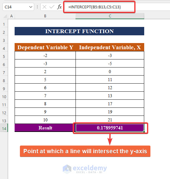
Consider the following scenario: You have a data set of some independent values (X) and some dependent values of (Y). But there is no linear relationship between X and Y like a straight line. Therefore, we will use the INTERCEPT function to calculate the value of a dependent variable when the independent variable is zero (0). The following formula is used here,
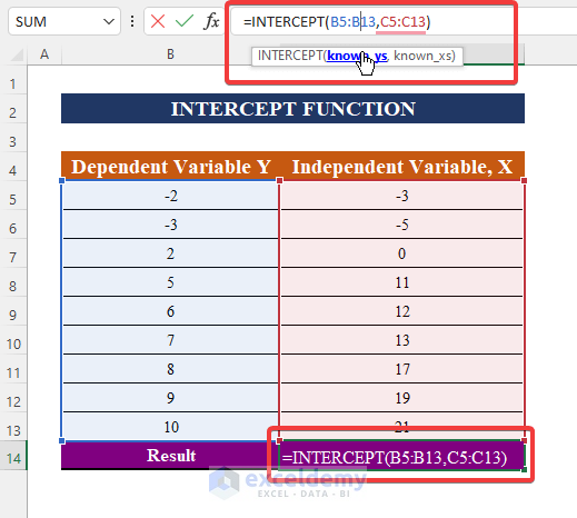
=INTERCEPT(B5:B13,C5:C13)Step 1:
- Type the INTERCEPT function in the cell C14
- Select the range B5:B13 for the dependent variable known_ys.
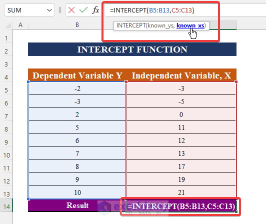
Step 2:
- Select the range C5:C13 for Independent variable known_xs.
Step 3:
- Press Enter to see the Result.

INTERCEPT Function: Regression Analysis
In the spreadsheet below, we will find the point where the linear regression line through the known x’s and known y’s crosses the y-axis.
Generally, the objective of a regression model is to figure out how predictors and responses are related. If this is the case, and X is never equal to 0, the intercept is of no use. It doesn’t tell you anything about X and Y’s relationship. Consider centering X when X never equals 0 but you want a meaningful intercept.
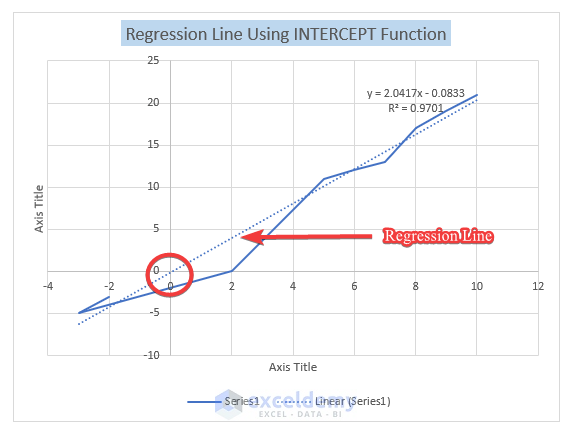
The intercept now has relevance if you rescale X so that the mean or any other relevant value = 0 (simply remove a constant from X). It’s the average value of Y at the specified X value. From the regression line, we have found that the intercept point from the regression analysis is relatable to the intercept point found from using the INTERCEPT function.
Read More: How to Find x-Intercept in Excel
✍ Things to Remember
✎ Numbers or names, arrays, or references containing numbers should be used as parameters.
✎ Text, logical values, and empty cells in an array or reference argument are ignored; however, cells with the value zero are included.
✎ INTERCEPT returns the #N/A error value if known ys and known xs have different numbers of data points or no data points.
Download Practice Workbook
Download this practice workbook to exercise while you are reading this article.
Conclusion
To conclude, I hope this article has given you some useful information about how to apply the INTERCEPT function in Excel. You should learn at first and then apply all of these procedures. Take a look at the practice workbook and put these skills to the test. Your valuable support keeps motivating us to make tutorials like this
If you have any questions – Feel free to ask us. Also, feel free to leave comments in the section below.
Stay with us & keep learning.
Excel INTERCEPT Function: Knowledge Hub
- How to Find Intercept of Two Lines in Excel
- How to Find Y Intercept in Excel
- How to Set Intercept Trendline in Excel
<< Go Back to Excel Functions | Learn Excel
Get FREE Advanced Excel Exercises with Solutions!
