How to Find Duplicate Rows Based on Multiple Columns in Excel

Method 1 – Using the COUNTIFS Function

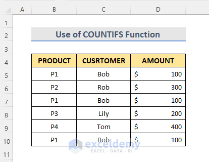
We will use the following dataset for this method.

STEPS:

• Select the cell range.
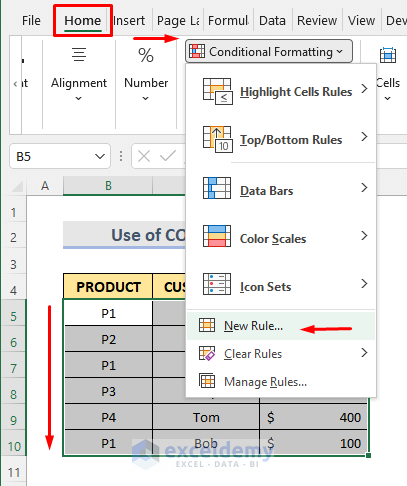
• Go to the Home tab and select the Conditional Formatting drop-down.
• Click on the New Rule option.

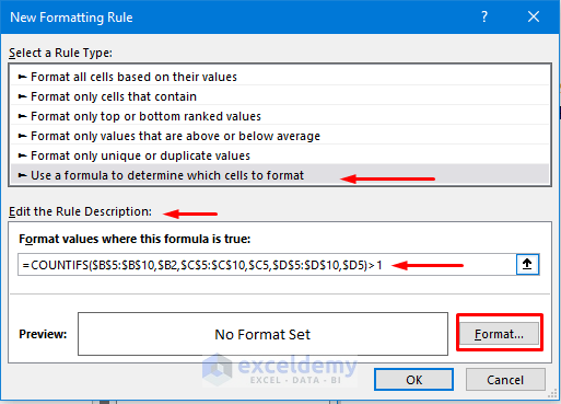
• A New Formatting Rule window pops up.
• Select a rule type ‘Use a formula to determine which cells to format’.
• Enter the following formula in the formula box:

• Select Format.

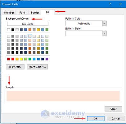
• A Format Cells window opens here.
• Go to the Fill option.
• From the Background Color group, select the color. We can see the sample of color in the Sample box.
• Click OK.

• Click OK.

We can see that all the duplicate rows are highlighted with the color we’ve selected before.

Read more: How to Find Duplicate Rows in Excel

Method 2 – Using the IF Function Based on Multiple Columns

We will use the following dataset for this method.

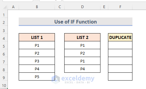
STEPS:

• Select Cell F5.
• Enter the following formula:

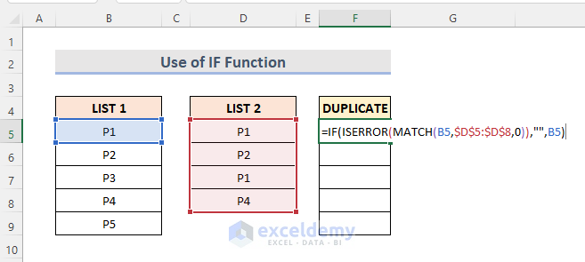
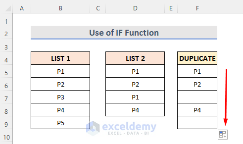
• Press Enter and use the Fill Handle tool to autofill the next cells.

How Does the Formula Work?

• MATCH(B5,$D$5:$D$8,0): This will return the position of Cell B5.
• ISERROR(MATCH(B5,$D$5:$D$8,0)): This will return the TRUE or FALSE value based on the presence of an error.
• IF(ISERROR(MATCH(B5,$D$5:$D$8,0)),”,B5): This will display the value if it meets the above criteria; otherwise, leave the cell blank.

Read more: How to Find Repeated Cells in Excel

Method  – Using the Array Formula 

We will use the following dataset for this method.

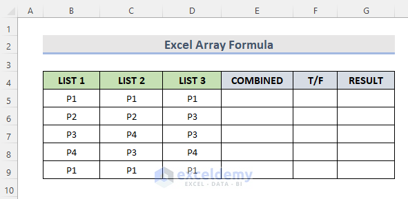
STEPS:

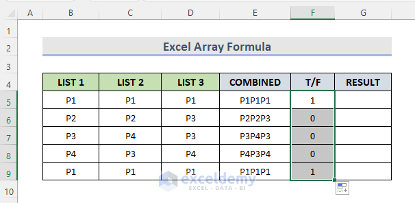
• Select Cell E5.
• Enter the following formula:

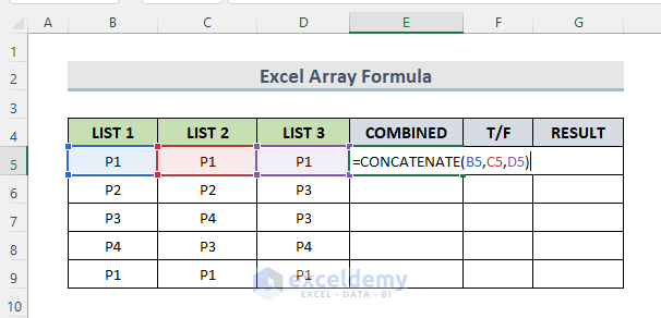
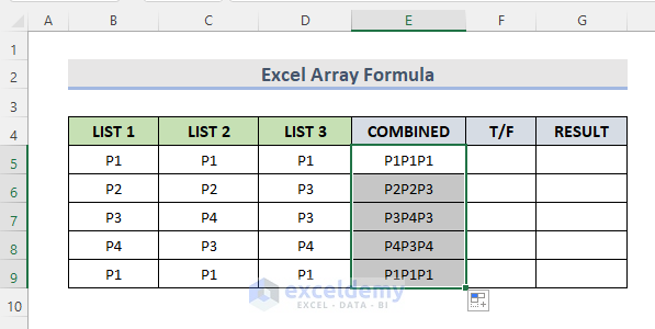
• Press Enter and use the Fill Handle. See the below result.

• Select cell F5.
• Enter the following formula:

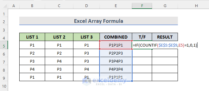
• Press Enter and use the Fill Handle tool for the cells below.

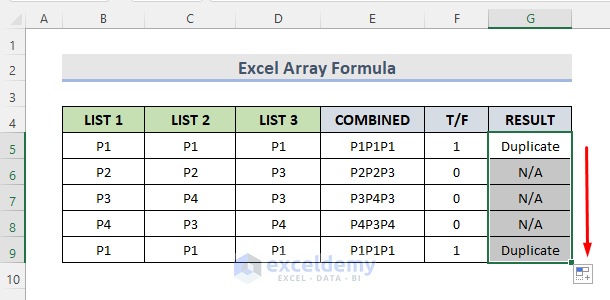
• Select cell G5.
• Enter the following formula:

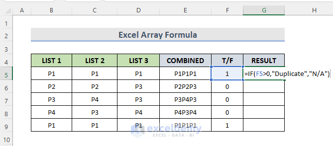
• Press Enter and use the Fill Handle tool to see the result.

How Do the Formulas Work?

• CONCATENATE(B5,C5,D5): This will combine the text of cells B5, C5 & D5.
• IF(COUNTIF($E$5:$E$9,E5)=1,0,1): The COUNTIF function will count the number of cells from the range E5:E9 for the cell E5. And the IF function will return the value ‘0’ if it’s TRUE and ‘1’ if it’s FALSE.
• IF(F5>0,”Duplicate”,”N/A”): This will return “Duplicate” if cell F5 is greater than ‘0’ and “N/A” if it’s not.

Read More: How to Find Repeated Numbers in Excel

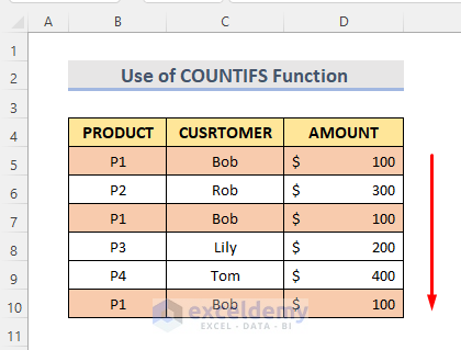
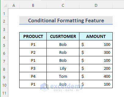
Method 4 – Using Conditional Formatting

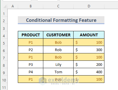
Here we have a dataset (B4:D10) of customers with their purchased products and amounts.

STEPS:

• Select the dataset.
• Go to the Home tab and click on the Conditional Formatting drop-down.
• Go to the Highlighted Cells Rules group and select Duplicate Values.

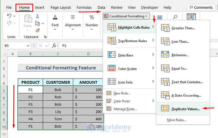
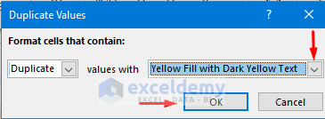
• The Duplicate Values message box pops up.
• From the drop-down menu, select the color that will indicate the duplicate cells.
• Click OK.

We can see all the duplicate rows in yellow filled with dark yellow text.

Read more: How to Filter Duplicates in Excel

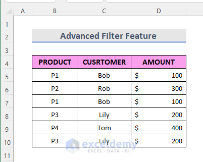
Method 5 – Using the Advanced Filter Feature 

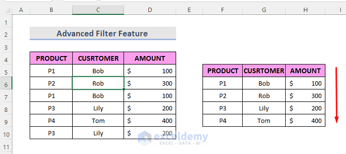
We will use the following dataset for this method.

STEPS:

• Select the cell range.
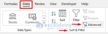
• Go to the Data tab.
• From the Sort & Filter group, select Advanced.

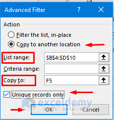
• An Advanced Filter window pops up.
• Check the box ‘Copy to another location.’
• Make sure the list range is already included in the data range.
• Select the cell reference in the Copy to box where we want to see the duplicate rows. Here we input Cell F5.
• Click on the ‘Unique records only’ option.
• Select OK.

We can see the dataset without duplicate rows in the range E5:H9.

Read More: How to Compare Rows for Duplicates in Excel

Method 6 – Using Excel VBA 

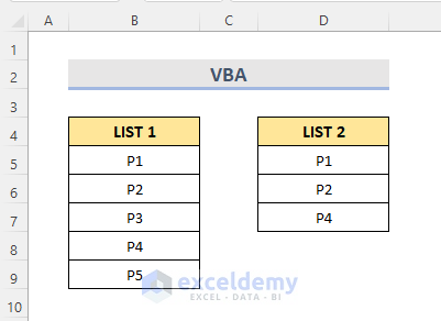
We will use the following dataset for this method.

STEPS:

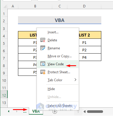
• Select the active worksheet from the sheet bar and right-click on it.
• Click on the View Code option.

• A VBA Module window opens. We can also open it by pressing the ‘Alt + F11’ keys. Click on Insert > Module.
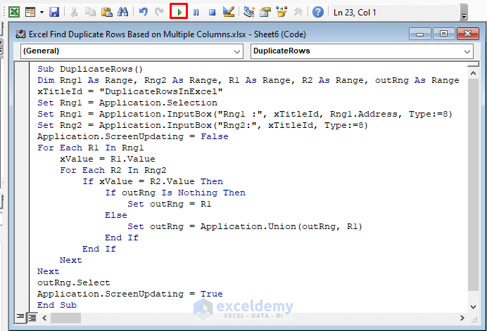
• Enter the following formula:

Sub DuplicateRows()
Dim Rng1 As Range, Rng2 As Range, R1 As Range, R2 As Range, outRng As Range
xTitleId = "DuplicateRowsInExcel"
Set Rng1 = Application.Selection
Set Rng1 = Application.InputBox("Rng1 :", xTitleId, Rng1.Address, Type:=8)
Set Rng2 = Application.InputBox("Rng2:", xTitleId, Type:=8)
Application.ScreenUpdating = False
For Each R1 In Rng1
xValue = R1.Value
For Each R2 In Rng2
If xValue = R2.Value Then
If outRng Is Nothing Then
Set outRng = R1
Else
Set outRng = Application.Union(outRng, R1)
End If
End If
Next
Next
outRng.Select
Application.ScreenUpdating = True
End Sub

• Click on the Run option or press the F5 key.

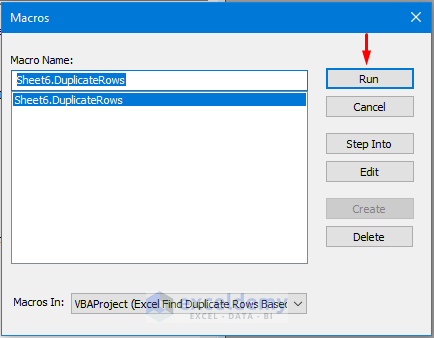
• A Macros confirmation box pops up. Select the sheet and click on Run.

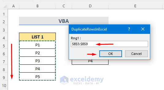
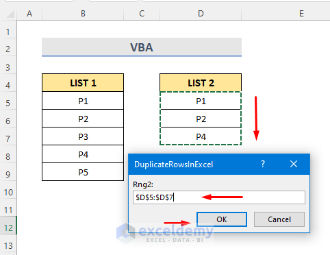
• We can see the DuplicateRowsInExcel message box. Here input the Rng1, in which we will highlight the duplicate rows from the worksheet.
• Select OK.

• Another DuplicateRowsInExcel message box pops up. Select the Rng2, which will be used as the finding column.
• Click OK.

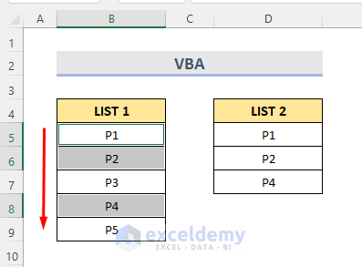
We can see the duplicate rows are highlighted in the LIST 1 column.

Read More: How to Compare Two Excel Sheets for Duplicates

Practice Workbook

Download the following workbook and practice.

Related Readings

• How to Find Matching Values in Two Worksheets in Excel
• How to Find Duplicates in Excel and Copy to Another Sheet
• Excel VBA to Find Duplicate Values in Range
• How to Find Duplicates in a Column Using Excel VBA
• How to Use VBA Code to Find Duplicate Rows in Excel

<< Go Back to Find Duplicates in Excel Column | Find Duplicates in Excel | Learn Excel