Method 1 – Find Duplicates in the Same Row but Different Columns to Compare Rows for Duplicates
Option 1 – Decide in a New Column to Show Duplicates for the Same Row
Steps:
- Under column header F, make a new column to show the result.
- Enter the following formula in cell F5.
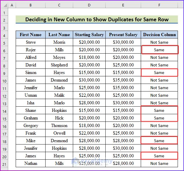
=IF(D5=E5,"Same","Not Same")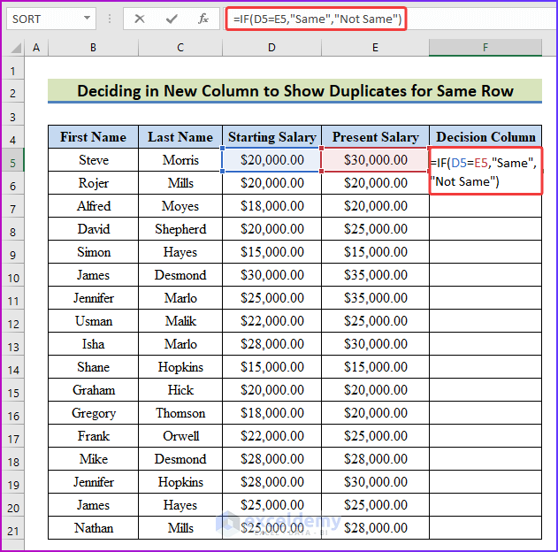
- Press Enter to see the comparisons for row 5.
- To get the desired results for the rest of the cells, use AutoFill.
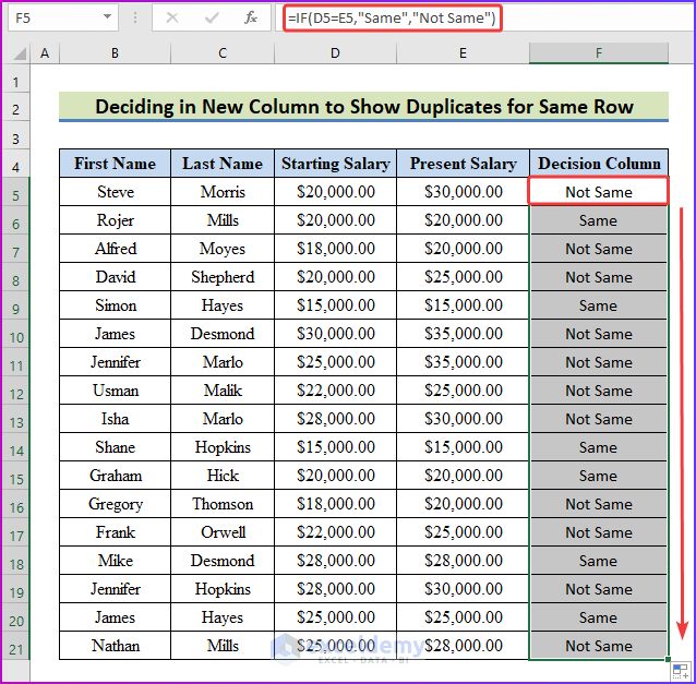
- After applying the formula, you will be able to see which particular row contain duplicates.
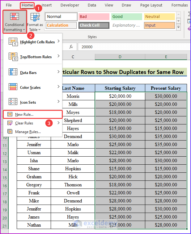
Option 2 – Highlight Particular Rows to Show Duplicates for Same Row
Steps:
- Select cell range D5:E21 from the primary data set.
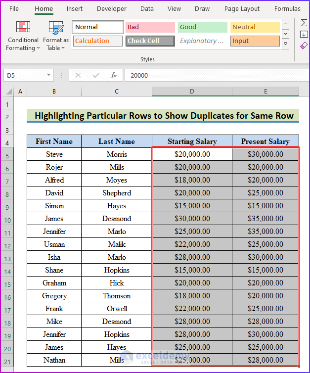
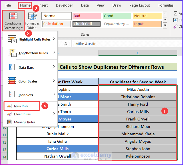
- Go to the Home tab of the ribbon and select Conditional Formatting.
- From the dropdown, choose New Rule.
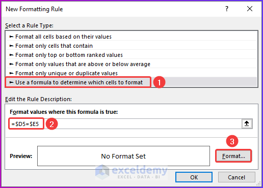
- The New Formatting Rule dialog box will open.
- To apply a formula, select Use a formula to determine which cells to format under the Select a Rule Type labels.
- In the type box, insert the following formula.
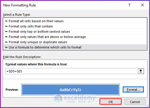
=$D5=$E5- Click on the Format.
- Configure the highlighted criteria and select OK to close the dialog box.
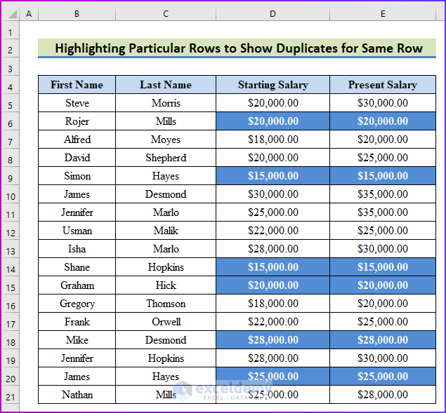
- You will be able to see the duplicates highlighted in the data set like the following image.
Read More: How to Find Duplicate Rows in Excel
Method 2 – Find Duplicates in Different Rows to Compare Rows for Duplicates
Option 1 – Create a Helper Column to Show Duplicates for Different Rows
Steps:
- Show which cell values have duplicates in different rows and enter the following formula in cell C5.
=IF(COUNTIF($D$5:$D$14,B5)>0,"Match","Don't Match")- The formula will help find out cell values that are present in both columns C and D but in different rows.
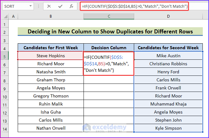
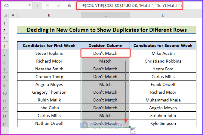
- Press Enter and use the Fill Handle to get the result.
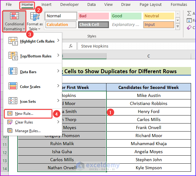
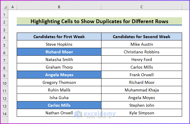
Option 2 – Highlight Cells to Show Duplicates for Different Rows
Steps:
- Select cell range B5:B14 and go to New Rule from Conditional Formatting.
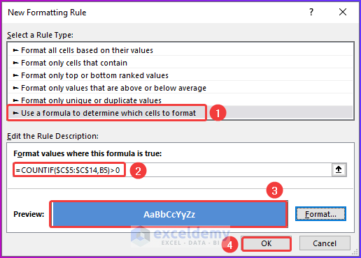
- In the box for applying a formula, insert the following formula.
=COUNTIF($C$5:$C$14,B5)>0- Set the highlighting criteria and press OK.
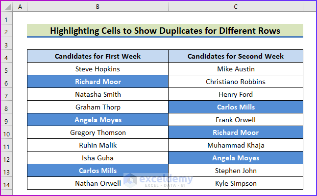
- This will highlight the values of column B that are also in column C.
- To highlight the duplicates in column C, select cell range C5:C14 and choose New Rule.
- Modify the formatting rule box and, in the box, insert the following formula.
=COUNTIF($C$5:$C$14,B5)>0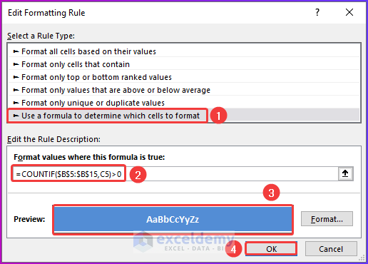
- Press OK.
Read More: How to Find Repeated Cells in Excel
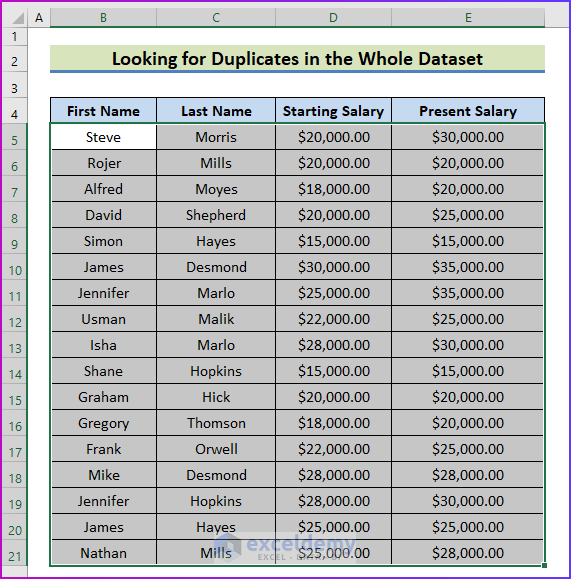
Method 3 – Look for Duplicates in the Whole Dataset
Steps:
- Select the data range B5:B21 to look for duplicates in the whole data set.
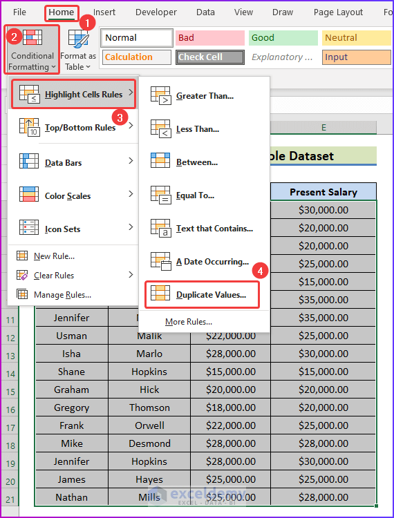
- Choose Conditional Formatting from the Home tab, and from the dropdown, select Highlight Cells Rules.
- From the second dropdown, choose Duplicate Values.
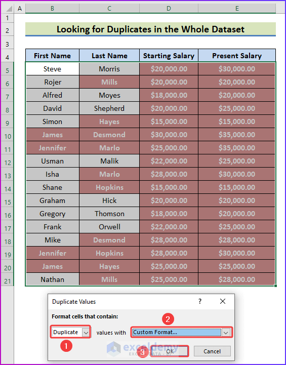
- In the Duplicate Values dialog box, set the criteria of formatting and select the text and fill color for the final result.
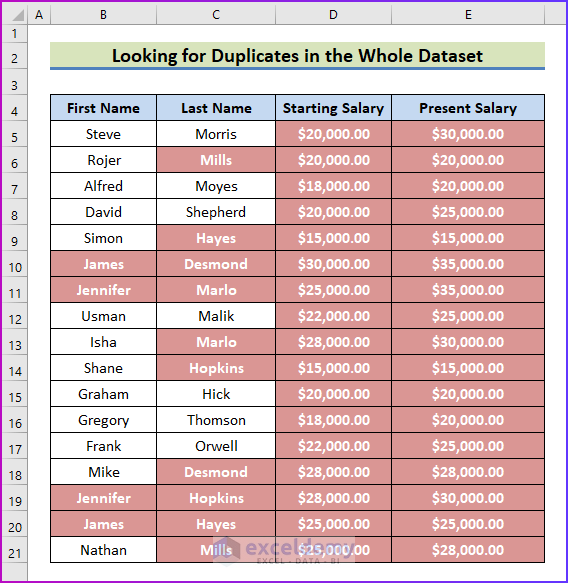
- The duplicate values in your cells will be highlighted like the following image.
Read More: How to Find Repeated Numbers in Excel
Find Duplicates in the Same Column in Excel
Option 1 – Decide in a New Column to Show Duplicates
Steps:
- Create a new column under column D.
- In cell D5, enter the following combination formula.
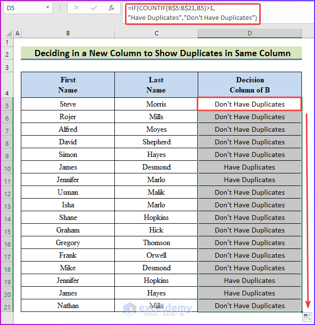
=IF(COUNTIF(B$5:B$21,B5)>1,"Have Duplicates","Don't Have Duplicates")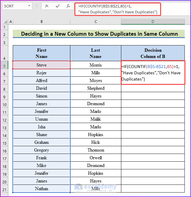
- Press Enter to get the result for the first cell value of column B.
- Drag the Fill Handle to show the results for the lower cells of the same column.
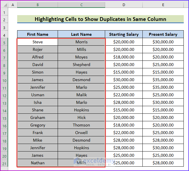
Option 2 – Highlight Cells to Show Duplicates
Steps:
- Select the cell range B5:C21 which includes both columns B and C.
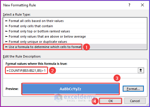
- Open the New Formatting Rule box from Conditional Formatting.
- In the box, enter the following formula.
=COUNTIF(B$5:B$21,B5)>1- Make all the formatting cells and press OK.
- You will find your selected data range highlighted like the following image where any duplicates in a single column will be highlighted.

Read More: How to Filter Duplicates in Excel
Things to Remember
- While inserting formulas in the assigned cells or in the dialog box of Conditional Formatting, give proper cell reference. Otherwise, you will not get the desired result.
- After inserting formulas in Conditional Formatting, remember to format cells to highlight the result.
Download the Practice Workbook
Further Readings
- Excel Find Duplicate Rows Based on Multiple Columns
- How to Compare Two Excel Sheets for Duplicates
- How to Find Matching Values in Two Worksheets in Excel
- How to Find Duplicates in Excel and Copy to Another Sheet
- Excel VBA to Find Duplicate Values in Range
- How to Find Duplicates in a Column Using Excel VBA
- How to Use VBA Code to Find Duplicate Rows in Excel
<< Go Back to Duplicates in Excel | Learn Excel
Get FREE Advanced Excel Exercises with Solutions!

Yoyo. Good stuff.
How do I get the largest number in the first column of Excel?
Hi Craig!
Just use the MAX function in the first column, you will get the largest number from the column.
Best regards