Let’s get introduced to the data table first. We have a table that has 3 columns and 14 rows. The columns are named Ship Mode, Province, and Customer Segment. 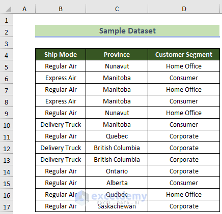
Method 1 – Using Remove Duplicates Tool
The quickest way to remove duplicates is to use the Remove Duplicates tool.
Steps:
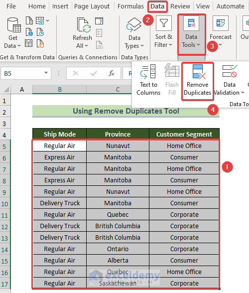
- Select your dataset
- Go to Data tab >> Data Tools group >> Remove Duplicates tool.
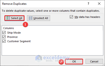
The Remove Duplicates pop-up will appear,
- Click on the Select All button, or you can filter according to your preference.
- Click on the OK button.
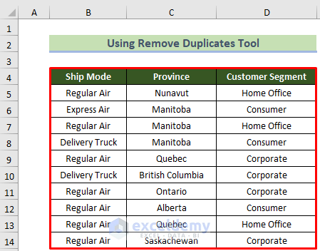
The following filtered data will appear.
Read More: How to Find Duplicate Rows in Excel
Method 2 – Using Advanced Filter Tool
Steps:
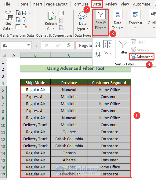
- Select your dataset.
- Select the Data tab >> Advanced option in the Sort & Filter group.
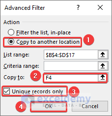
The Advanced Filter pop-up will appear.
- Select Copy to another location.
- Select the data table as the list range.
- Select the destination position in the Copy to: text box.
- Tick Unique records only.
- Click on the OK button.
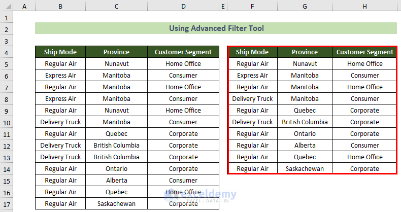
As a result, the following filtered data table will appear.
Read More: How to Find Repeated Cells in Excel
Method 3 – Using Pivot Table
Steps:
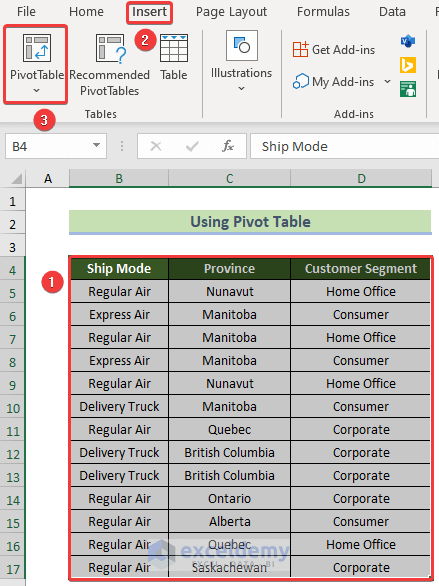
- After selecting the data table, click on the Pivot Table option under the Insert tab.
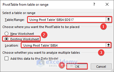
The PivotTable from table or range window will appear
- Select the options as shown below:
As we are replacing previous data with new pivot table data, a Microsoft Excel warning box will appear.
- Click OK.

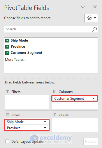
The PivotTable and PivotTable Fields pane will appear.
- Drag the Ship Mode and Province fields to the Rows area and Customer Segment to the Columns area. Or other fields of your choice.
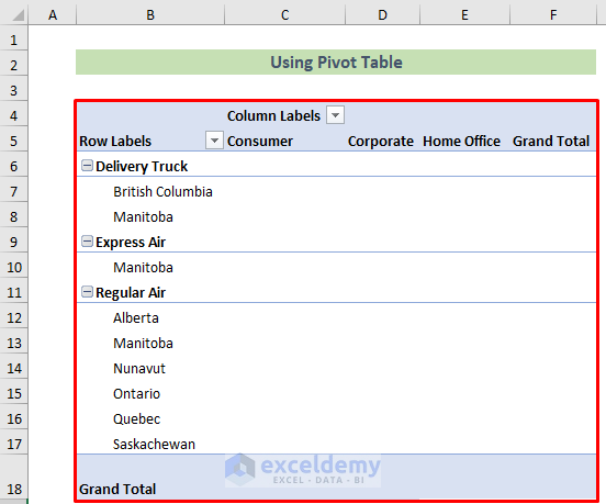
The filtered data will appear on the left side.
Read More: How to Find Repeated Numbers in Excel
Method 4 – Using Power Query
Steps:
- Select your dataset.
- Select the From Table/Range option under the Data tab.
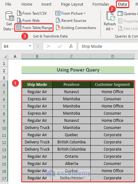
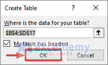
- Select the data range.
- Tick My table has headers.
- Click the OK button.
A Power Query Editor will appear, where the table will be formed.
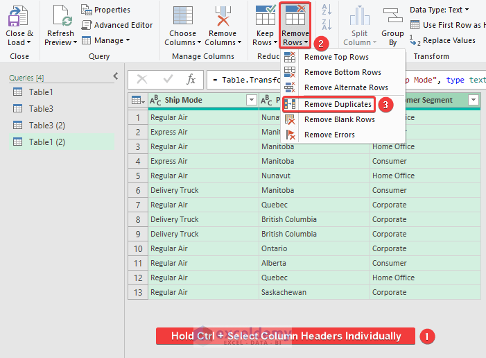
- Hold down the Ctrl key and select the table’s columns individually.
- Under the Home tab, select the Remove Duplicates option under the Remove Rows tool.
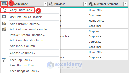
The filtered table will appear.
- Click on Copy Entire Table.
- Close the Power Query Editor window.
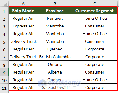
The filtered table as specified appears.
Read More: How to Compare Rows for Duplicates in Excel
Method 5 – Using CONCATENATE and COUNTIFS Functions
Steps:
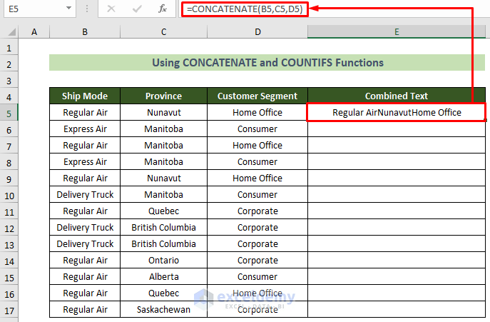
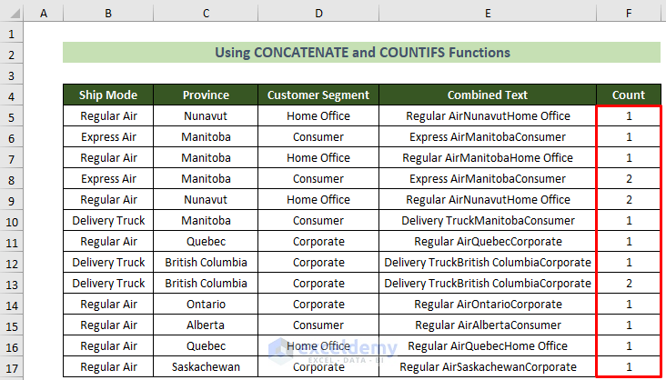
This method requires joining all of the texts in a row using the CONCATENATE function into a new column named Combined Text.
- Click on cell E5 and insert the following formula:
=CONCATENATE(B5,C5,D5)- Press Enter.
- Place your mouse cursor on the bottom right position of the cell and drag the fill handle down to Autofill the rest of the column.
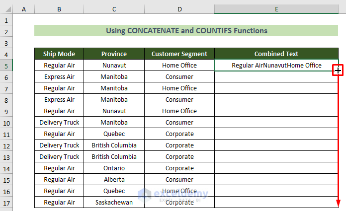
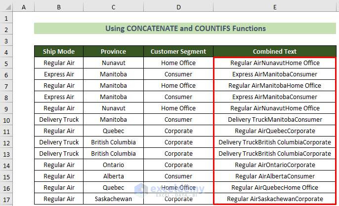
The combined text will form as below.
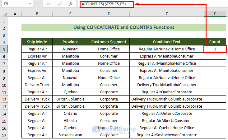
- Click on cell F5 and insert the following formula:
=COUNTIFS($E$5:E5,E5)- Press Enter.
- Use the fill handle to copy the formula to the rest of the column.
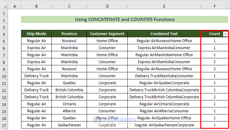
A Count column will be created.
- Select the Count column.
- Go to the Home tab >> Editing group >> Sort & Filter tool >> Filter option.
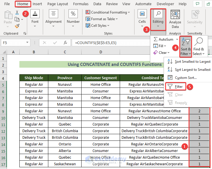
- Click on filter 1 only, because only number 1 here contains the unique data.
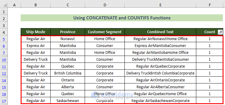
The following filtered table will be formed:
Read More: Excel Find Duplicate Rows Based on Multiple Columns
Method 6 – Using Dynamic Array Formula
Steps:
We’ll use the UNIQUE function, which returns unique values by filtering duplicates.
- Click on cell B5 and insert the following formula:
=UNIQUE('Sample Dataset'!B5:D17,FALSE,FALSE)- Press Enter.
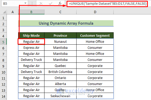
The table containing filtered data will be returned.
Read More: How to Compare Two Excel Sheets for Duplicates
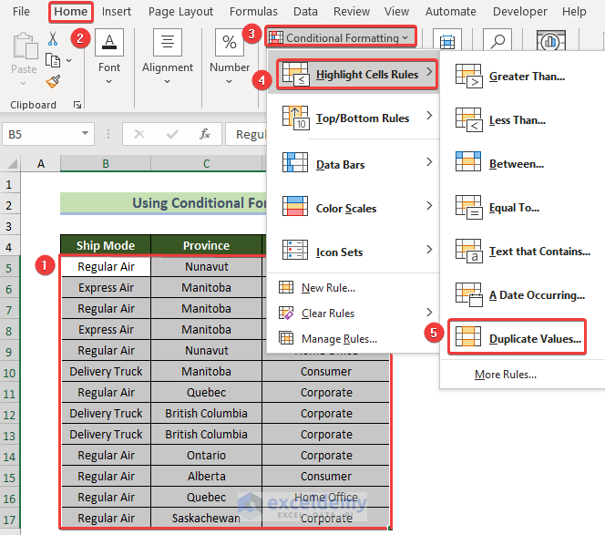
Method 7 – Applying Conditional Formatting
Steps:
- Select the data table range.
- Go to the Home tab.
- From the Conditional formatting drop-down, select Duplicate Values under Highlight Cells Rules.
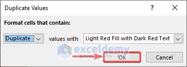
The Duplicate Values pop-up will appear.
- Select the Duplicate option and formatting of your choice.
- Select the Province column, as it is the only column with a unique value.
- Go to the Home tab >> Editing group >> Sort & Filter tool >> Filter option.
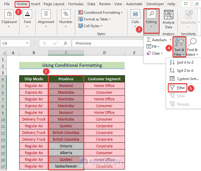
- Click on the Filter button.
- Select Filter by Color.
- Select No Fill for option Filter by Cell Color.
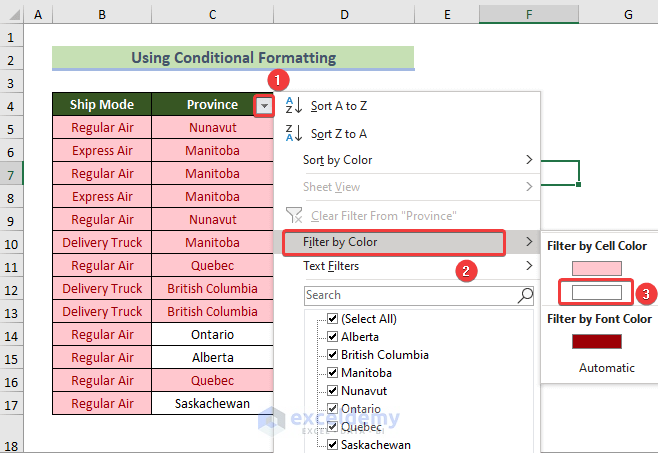
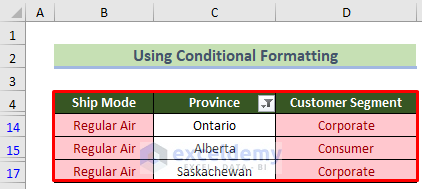
The following filtered table will be formed.
Read More: How to Find Matching Values in Two Worksheets in Excel
Download Practice Workbook
Related Contents
- How to Find Duplicates in Excel and Copy to Another Sheet
- Excel VBA to Find Duplicate Values in Range
- How to Find Duplicates in a Column Using Excel VBA
- How to Use VBA Code to Find Duplicate Rows in Excel
<< Go Back to Find Duplicates in Excel | Learn Excel
Get FREE Advanced Excel Exercises with Solutions!

greatttttt
thankssssss