How to Find Matching Values in Two Worksheets in Excel

Method 1 – Using the EXACT Function in Excel to Find Matching Values in Two Worksheets

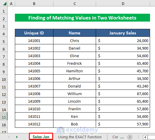
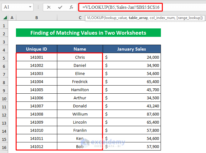
We have two different datasets in two worksheets. The dataset contains the columns named “Unique ID”, “Name”, and “Salary” of some sales reps. We’ll find matching values that are present in both worksheets. The “Sales-Jan” worksheet is shown below.

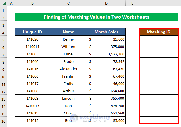
Here’s the next dataset. We put a “Matching ID” column to display the results.

Steps:

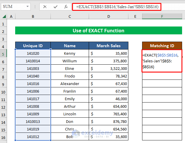
• In cell F5, apply the following function.

• Insert the values so it looks like the following:

Text1 is $B$5:$B$16 as we want to find the matching IDs between two worksheets. Text2 is ‘Sales-Jan’!$B$5:$B$16 which is the Unique ID column in Sales-Jan.

• Press Enter to get the result.

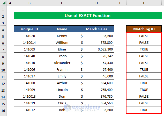
• The EXACT function is returning FALSE when the value is not matched and TRUE for those values which are matched.

Read More: How to Find Duplicate Rows in Excel

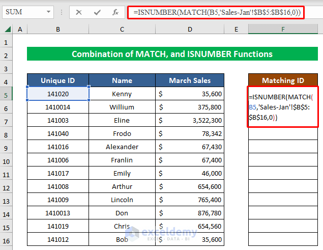
Method 2 – Combining MATCH with the ISNUMBER Function to Get Matching Values

Steps:

• In cell F5, apply the following formula:

Lookup_values is B5, Lookup_array is ‘Sales-Jan’!$B$5:$B$16 (You can click on the Sales-Jan worksheet to go there and select the array). [match_type]is EXACT (0).

• Hit Enter.

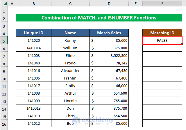
• The formula will give you “TRUE” if the values are matched.
• Apply the same formula via AutoFill for the rest of the cells to get the final result.

Read More: How to Find Repeated Cells in Excel

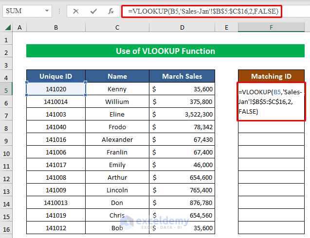
Method 3 – Inserting the VLOOKUP Function to Find Matching Values in Two Worksheets

Steps:

• Use the following function in F5:

• Col_index_num is 2. We want to get the matching names with the matching IDs
• [range_lookup]value is FALSE (Exact)

• Press Enter to get the result.

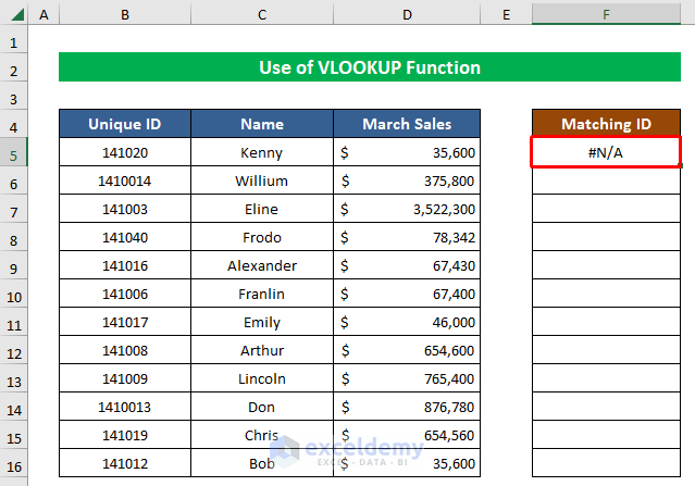
• Apply the same function to the rest of the cells to get the final result. When the VLOOKUP doesn’t find the matching values, it will return the #N/A error.

Read More: How to Find Repeated Numbers in Excel

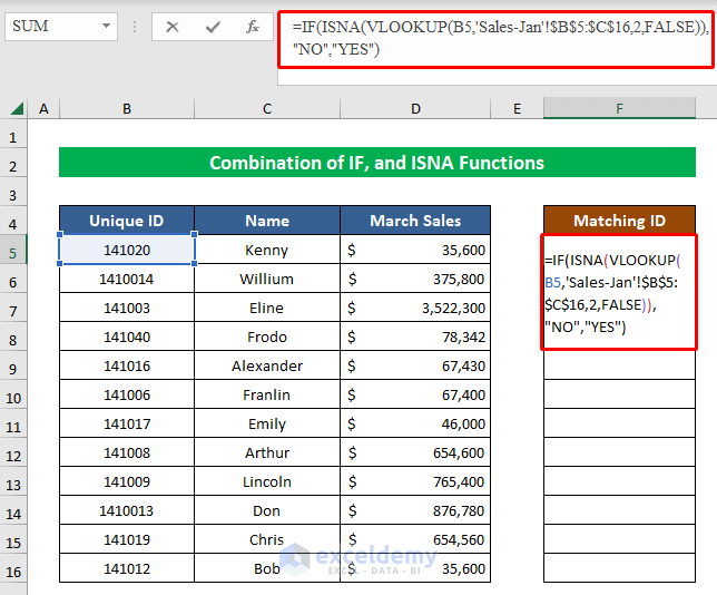
Method 4 – Merging IF with ISNA to Obtain Matches from Two Worksheets

Steps:

• Use the following formula in F5:

• If the values are matched, the formula will return YES. Otherwise, it will return NO.

• Apply the function by pressing Enter.

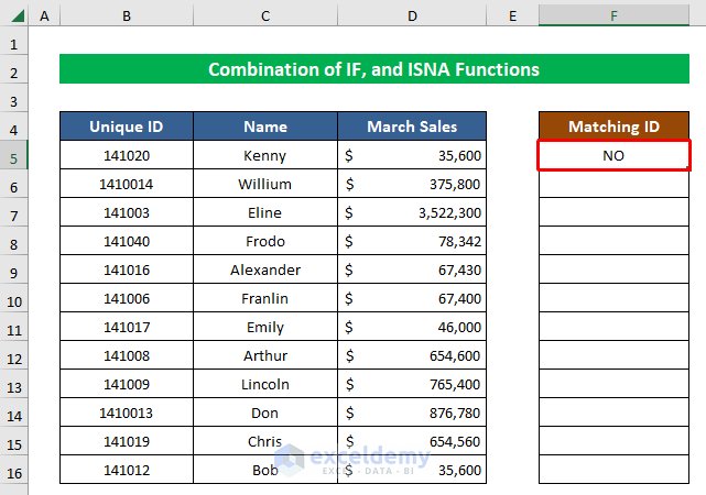
• Apply the same formula to the rest of the cells via AutoFill to get the final result.

Read More: How to Filter Duplicates in Excel

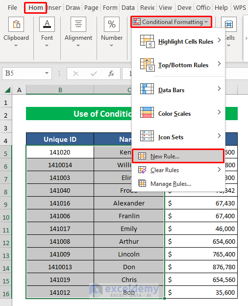
Method 5 – Using Conditional Formatting to Find Matching Values in Two Worksheets

Steps:

• Choose cells (B5:C16) and select New Rule from the Conditional Formatting section.

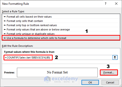
• In the New Formatting Rule window, choose Use a formula to determine which cells to format.
• Insert the following formula into the box.

• Click Format.

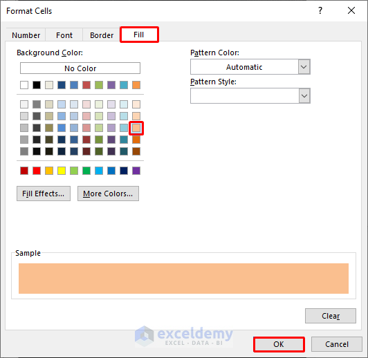
• Choose a color from Fill and hit OK.

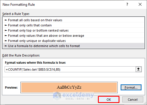
• Click OK to finish.

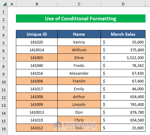
• This highlights all matching values.

Read More: How to Compare Rows for Duplicates in Excel

Things to Remember

• The EXACT function is case-sensitive. It won’t see Alexander and alexander as being a match.
• The VLOOKUP function always searches for lookup values from the leftmost top column to the right. This function never searches for the data on the left.
• When you select your Table_Array, you have to use absolute cell references ($) to block it from being modified via AutoFill.

Download the Practice Workbook

Similar Articles for You to Explore

• Excel Find Duplicate Rows Based on Multiple Columns
• How to Compare Two Excel Sheets for Duplicates
• How to Find Duplicates in Excel and Copy to Another Sheet
• Excel VBA to Find Duplicate Values in Range
• How to Find Duplicates in a Column Using Excel VBA
• How to Use VBA Code to Find Duplicate Rows in Excel

<< Go Back to Find Duplicates in Excel | Learn Excel