Method 1 – Viewing Two Excel Sheets Side by Side to Find Duplicates
Let’s consider we have an Excel workbook with two sheets. Here, we will compare them by viewing them side by side.
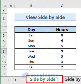
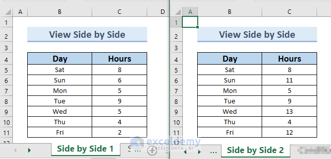
The first sheet is Side by Side 1.
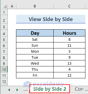
And the second sheet is Side by Side 2.
We have duplicates in the two sheets. We will find these duplicates by viewing them side by side.
Steps:
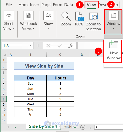
- Open the workbook, click the View tab>> from Window >> click New Window.
- The same workbook will open in two windows.
- Go to the View tab >> from Windows >> select Arrange All.
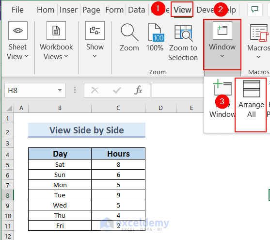
- An Arrange Windows dialog box will appear with several options.
- Select Vertical >> click OK.
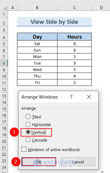
You can see two sheets side by side and you can compare two Excel sheet duplicates.
Read More: How to Find Duplicate Rows in Excel
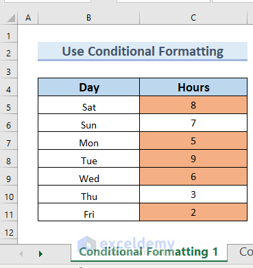
Method 2 – Using Conditional Formatting to Compare Two Excel Sheets for Duplicates
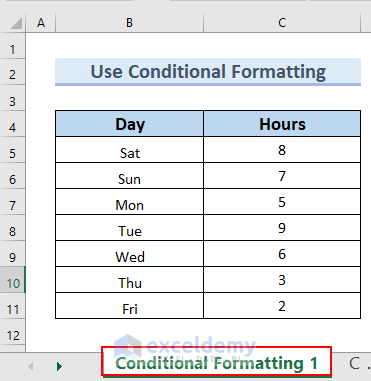
The first sheet is Conditional Formatting 1.
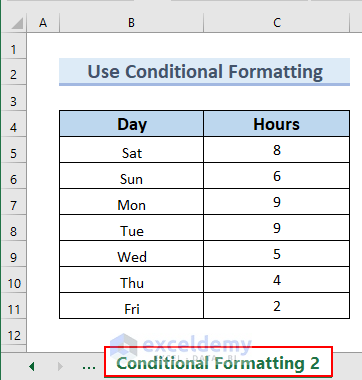
And the second sheet is Conditional Formatting 2.
We have duplicates in the two sheets. We will find these duplicates by using Conditional Formatting.
Steps:
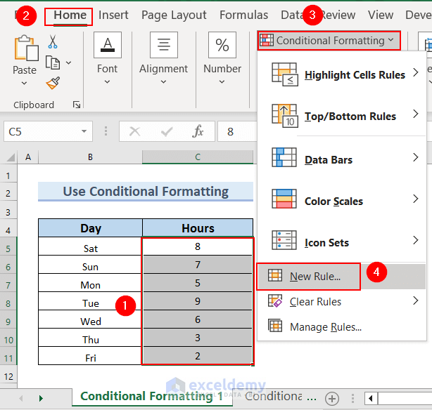
- Select the cells you want to apply Conditional Formatting. We selected cells C5:C11.
- Go to the Home tab >> Select Conditional Formatting.
- Select New Rule.
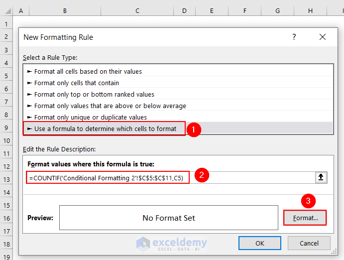
- A New Formatting Rule dialog box will appear.
- Select Use a formula to determine which cells to format option.
- Enter the following formula in the Format values where this formula is true box:
=COUNTIF('Conditional Formatting 2'!$C$5:$C$11,C5This formula includes the COUNTIF Function, which has two criteria. For the range, go to the second sheet. Select all the data from where we are looking and press F4 to make it absolute. Now, put a comma and specify the criteria. We will go to the first sheet and select the cell for that.
- Click Format.
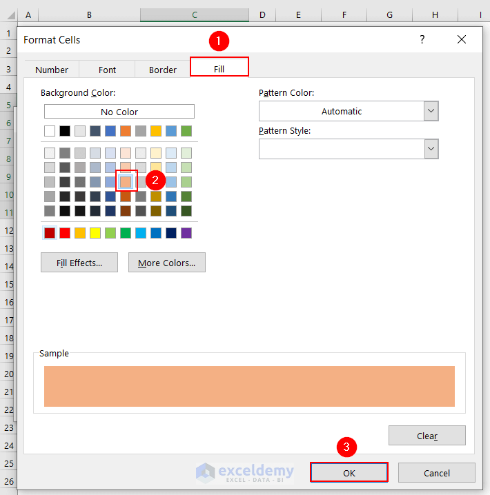
- A Format Cells dialog box will appear.
- From Fill >> select a color. We Choose Pink.
- You can see the Sample of the color.
- Click OK.
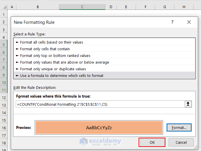
- You can see the Preview color in the New Formatting Rule dialog box.
- Click OK.
- Now, the final result is here, and we can see that the duplicate values are highlighted with Pink in the Conditional Formatting 1 sheet.
Read More: How to Find Repeated Cells in Excel
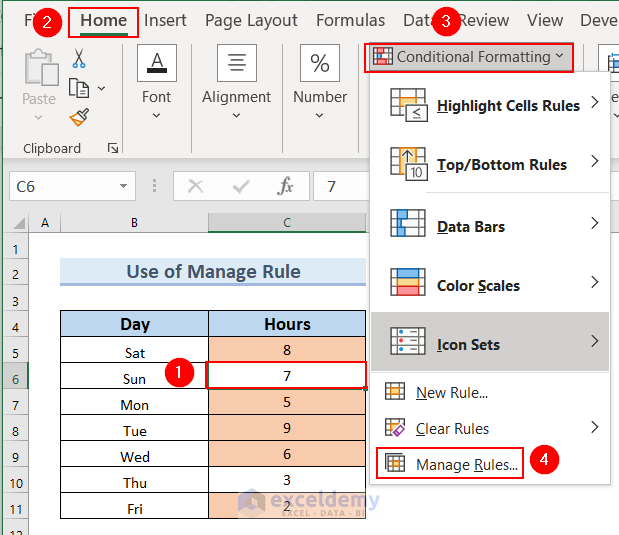
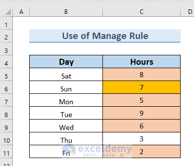
Method 3 – Using the Manage Rule in Conditional Formatting
Steps:
- Select a cell and go to the Home tab.
- Click on the Conditional Formatting and select Manage Rule.
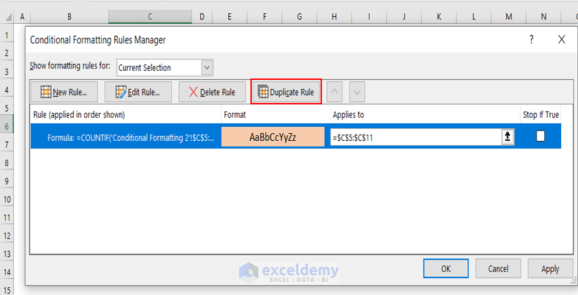
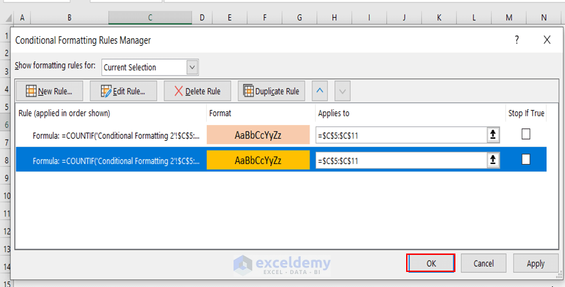
- A Conditional Formatting Rules Manager dialog box will appear.
- Select the Rule bar and click Duplicate Rule.
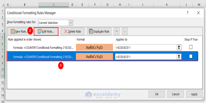
- A new Rule bar appeared >> Select it and click Edit Rule.
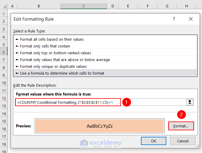
- An Edit Formatting Rule dialog box will appear.
- Add ‘>1’ with the formula.
- The formula becomes:
=COUNTIF('Conditional Formatting 2'!$C$5:$C$11,C5>1- Click on Format.
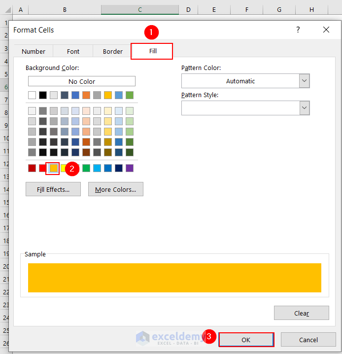
- A Format Cells dialog box will appear.
- From Fill >> select a color. We choose Orange.
- You can see the Sample of the color.
- Click OK.
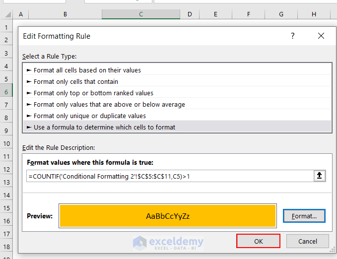
- You can see the Preview of the color in the Edit Formatting Rule dialog box.
- Click OK.
- Click OK in the Conditional Formatting Rules Manager dialog box.
- You can see the duplicate in cell C6 is highlighted with an Orange color.
Read More: How to Find Repeated Numbers in Excel
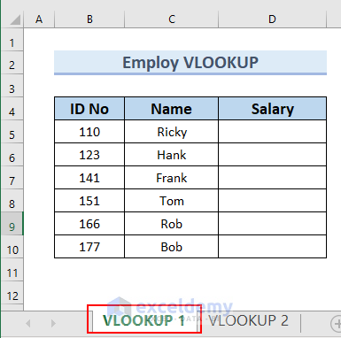
Method 4 – Inserting Excel VLOOKUP to Find Matches in Different Worksheets
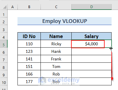
The first sheet is VLOOKUP 1, and we will pull the Salary from the second sheet.
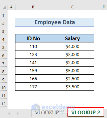
The second sheet is Vlookup 2.
Steps:
- Enter the following formula in cell C5 of the first sheet:
=IFERROR(VLOOKUP(B5,'VLOOKUP 2'!B5:C10,2,FALSE),"Not Available")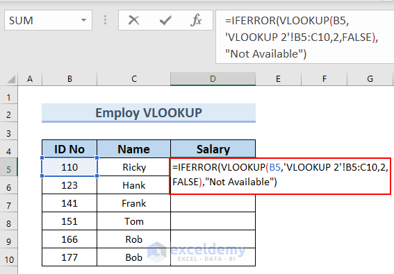
Formula Breakdown
- The VLOOKUP function searches for a value in a range of cells based on a lookup value.
- The IFERROR function makes sure no error comes if the formula contains any error.
- IFERROR(VLOOKUP(B5,’VLOOKUP 2′!B5:C10,2,FALSE),”Not Available”) → becomes
- Output: $4000
- Explanation: $4000 is the Salary for ID No 110.
- Press ENTER.
- Drag down the formula with the Fill Handle tool.
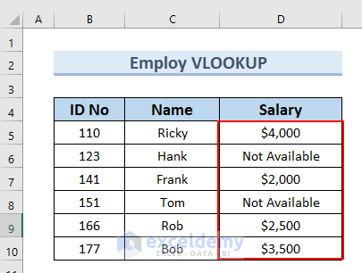
- You can see the complete Salary column.
- Not Available indicates no Duplicates for those ID No in the second sheet.
Read More: How to Filter Duplicates in Excel
Method 5 – Creating VBA Macro in Excel to Compare Two Sheets for Duplicates
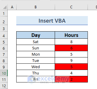
Here, you can see the data in VBA 1 sheet.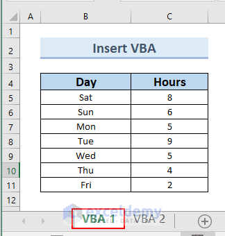
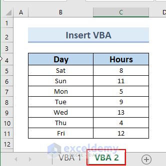
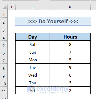
You can see the data set in VBA 2 sheet. These two sheets have duplicate values.
Steps:
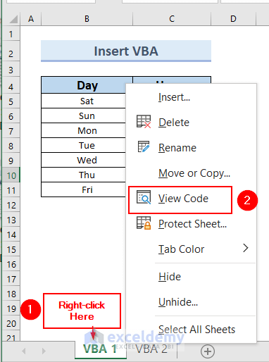
- Right-click on the VBA 1 sheet >> Select View Code from the Context Menu.
- A VBA Editor window will appear.
- Enter the following code in the window:
Sub Compare_Sheets_Duplicates()
Dim range_cell As Range
For Each range_cell In Worksheets("VBA 1").UsedRange
    If Not range_cell = Worksheets("VBA 2").Cells _
    (range_cell.Row, range_cell.Column) Then
     range_cell.Interior.Color = vbRed
   End If
Next range_cell
End Sub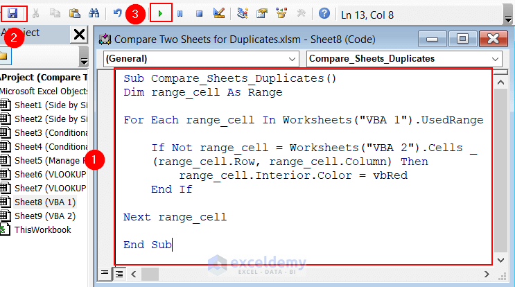
Code Breakdown
- We take Comapre_Sheets_Duplicates as the Sub.
- We declare range_cell as Range.
- We used the For loop to find the duplicates until the last cell.
- IF statement is used to color the cells that are not duplicates.
- Save the code >> Run the code.
- Go back to your Worksheet VBA 1.
- You can see that the cells that have no duplicates are marked with Red color.
- The unlighted cells are duplicates.
Read More: How to Compare Rows for Duplicates in Excel
Practice Section
You can download the above Excel file and practice.
Download the Practice Workbook
You can download the Excel file and practice.
Related Articles
- Excel Find Duplicate Rows Based on Multiple Columns
- How to Find Matching Values in Two Worksheets in Excel
- How to Find Duplicates in Excel and Copy to Another Sheet
- Excel VBA to Find Duplicate Values in Range
- How to Find Duplicates in a Column Using Excel VBA
- How to Use VBA Code to Find Duplicate Rows in Excel
<< Go Back to Learn Excel
Get FREE Advanced Excel Exercises with Solutions!

Thanks for informative article in finding duplicates in one file. Could you please explain how can we perform this method, if our data is in two different files?
You can check this article- How to Find Duplicate Values Using VLOOKUP in Excel