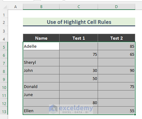
Method 1 – Use the Conditional Formatting ‘Highlight Cell Rules’ Option If a Cell Is Not Blank
Steps:
- Select the entire dataset B5:D13.
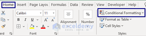
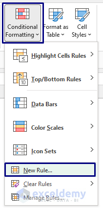
- Go to Home and select Conditional Formatting (in the Styles group).
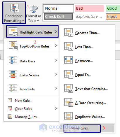
- From the Conditional Formatting drop-down, go to Highlight Cell Rules and pick More Rules.
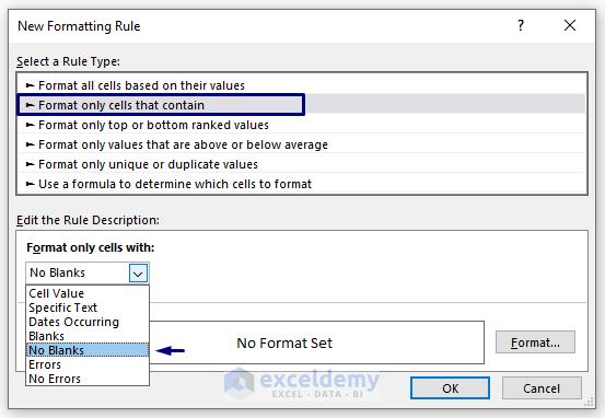
- The New Formatting Rule window will show up. The Format only cells that contain option is selected by default.
- Choose the No Blanks option from the Format only cells with drop-down.
- Click on Format.
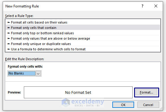
- Choose the highlight color from the Fill tab.
![]()
- Click OK and OK again to close both dialog boxes.
- You will see all the cells containing data have been highlighted.
![]()
Read More: How to Apply Conditional Formatting for Blank Cells in Excel
Method 2 – Apply a Simple Arithmetic Formula to Conditional Format a Cell
Steps:
- Select the entire dataset B5:D13.
- Go to Home, then to Conditional Formatting, and select New Rule.
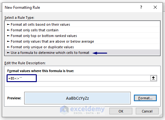
- The New Formatting Rule window will show up. Choose Rule Type: Use a formula to determine which cells to format.
- Insert the following formula under Format values where this formula is true.
=B5<>""- Click on the Format button and choose the highlight color from the Fill section.
- Click OK twice to close the dialog boxes.
![]()
Read More:Applying Conditional Formatting for Multiple Conditions in Excel
Method 3 – Appy the LEN Function in Conditional Formatting for Non-Blank Cells
Steps:
- Select the entire dataset B5:D13.
- Go Conditional Formatting and select New Rule.
- The New Formatting Rule window will show up. Choose Rule Type: Use a formula to determine which cells to format.
- Use the following formula for Format values where this formula is true.
=LEN(B5)>0- Go to Format and choose the highlight color from the Fill tab.
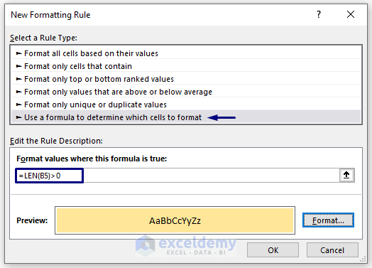
The LEN function returns the number of characters in a string, so a number greater than zero implies that the cell is not blank. Conditional Formatting then highlights the cell.
- Click OK twice to close the dialog boxes.
![]()
Related Content: Excel Conditional Formatting Formula
Method 4 – Use Excel NOT and ISBLANK Functions in Conditional Formatting
Steps:
- Select the entire dataset B5:D13.
- Go to Conditional Formatting and choose New Rule.
- The New Formatting Rule window will show up. Select Use a formula to determine which cells to format.
- Use the following formula under Format values where this formula is true.
=NOT(ISBLANK(B5))- Go to Format and choose the highlight color from Fill.
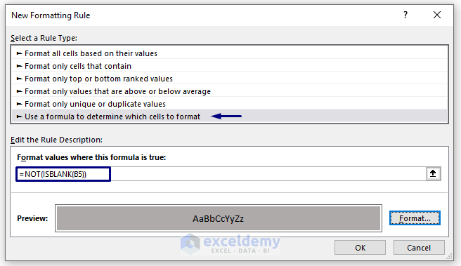
The ISBLANK function checks whether the cell is blank (which returns FALSE for non-blank cells). The NOT function reverts the result of the ISBLANK formula so FALSE is converted to TRUE. Conditional Formatting will end up highlighting cells that are not blank.
- Click OK twice to close the dialog boxes.
![]()
Related Content: How to Use Conditional Formatting in Excel
Download the Practice Workbook
Related Articles
- How to Format Cell Based on Formula in Excel
- How to Use Conditional Formatting Based on VLOOKUP in Excel
- How to Apply Conditional Formatting with INDEX-MATCH in Excel
- Excel Conditional Formatting Formula with IF
- Excel Conditional Formatting Formula If Cell Contains Text
- How to Change Text Color Based on Value with Excel Formula
- Conditional Formatting Multiple Text Values in Excel
- Conditional Formatting Entire Column Based on Another Column in Excel
- Excel Highlight Cell If Value Greater Than Another Cell
<< Go Back to Conditional Formatting with Multiple Conditions | Conditional Formatting | Learn Excel
Get FREE Advanced Excel Exercises with Solutions!

Which method is best?
Hi JEFF,
Thanks for your concern. Actually, all the methods here explained are very easy to understand. Considering the situation, you have to choose the best-suited method for serving your purpose. If you don’t want to use any formula, then you can use Method 1.
Regards,
Rafiul | ExcelDemy Team