Conditional Formatting Based On Another Cell Range in Excel

Here’s an overview of using Conditional Formatting based on another cell range.

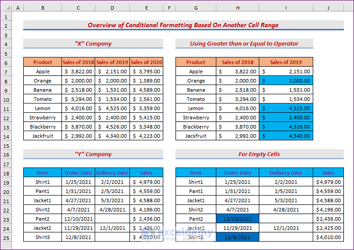
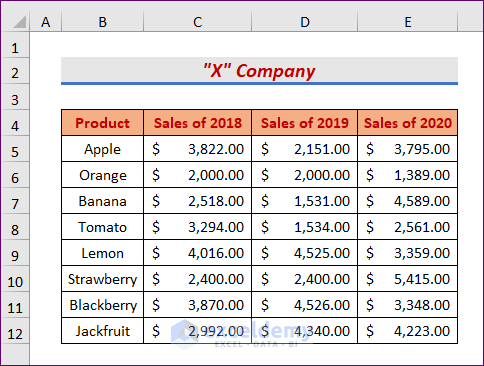
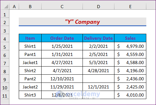
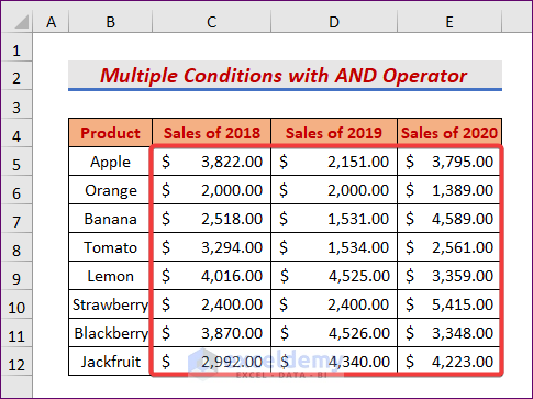
We have two data tables. The first table has Sales values for different years for some products and the second table contains Order Date, Delivery Date and Sales for some items of a company.

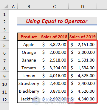
Method 1 – Conditional Formatting Based on Another Cell Range with the Equal to Operator

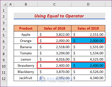
We will highlight the cells of the Sales of 2019 column based on the cell ranges of the Sales of 2018 column. For Conditional Formatting, the condition would be that the cells of the Sales of 2019 column will be Equal to the cell ranges of the Sales of 2018 column.

Step 1:

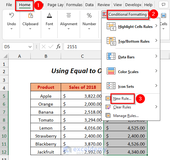
• Select the cell range on which you want to apply the Conditional Formatting (We have selected the column Sales of 2019).
• Go to the Home tab, select Conditional Formatting, and choose New Rule.

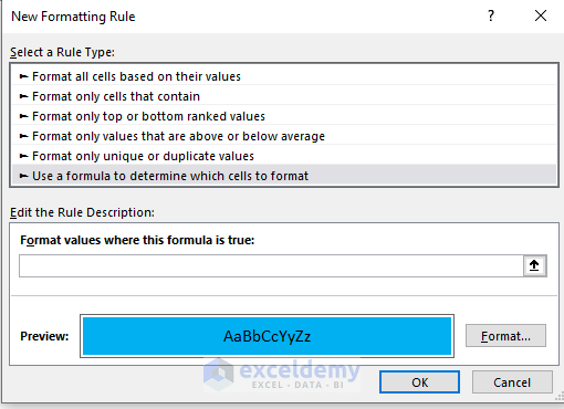
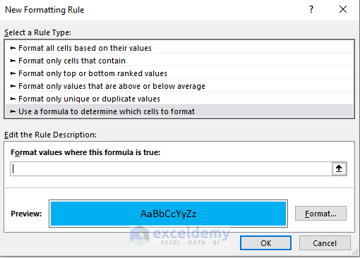
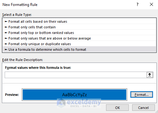
The New Formatting Rule Wizard will appear.

• Select Use a formula to determine which cells to format.

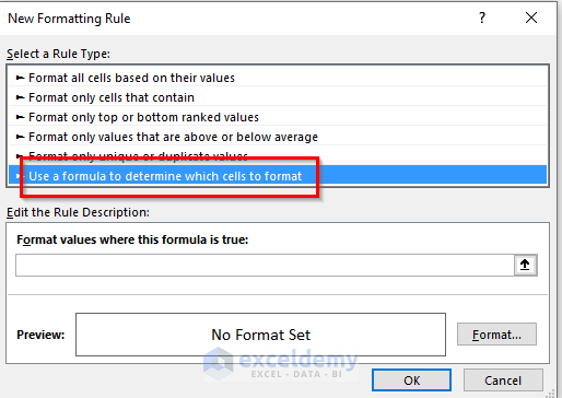
• Click on Format.

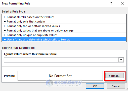
The Format Cells dialog box will open up.

• Select the Fill tab.
• Choose any Background Color.
• Click on OK.

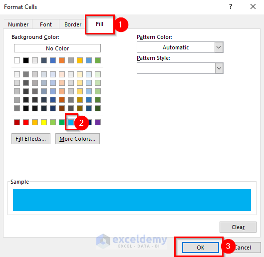
The Preview will be shown.

Step 2:

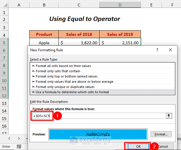
• Use the following formula in the Format values where this formula is true box:

When the cells of Column D are Equal to the corresponding cells of Column C, then the Conditional Formatting will appear in that cell of Column D.

• Press OK.

Result:

Read More: How to Do Conditional Formatting Based on Another Cell in Excel

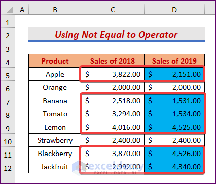
Method 2 – Conditional Formatting Based on Another Cell Range for Not Equal to

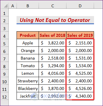
You can apply Conditional Formatting to the cells of the Sales of 2019 column by using Not Equal to Operator.

Steps:

• Follow Step 1 of Method 1.
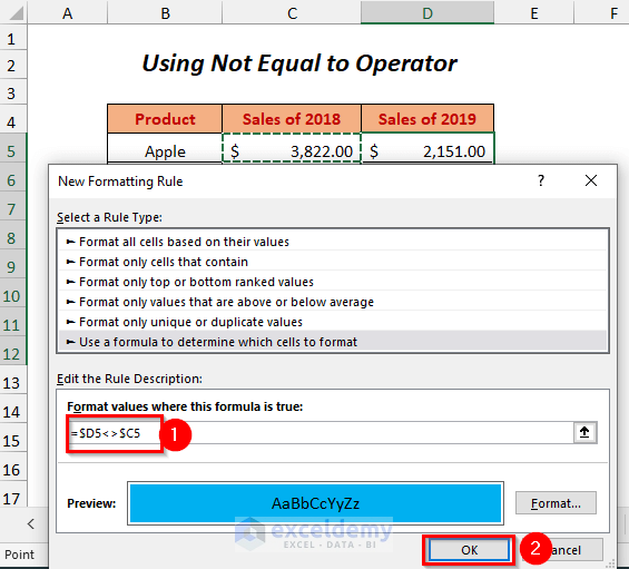
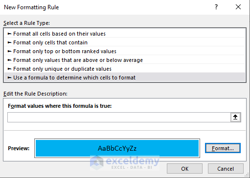
  You will get the following New Formatting Rule dialog box.

• Use the following formula in the Format values where this formula is true box.

When the cells of Column D are Not Equal to the corresponding cells of Column C, then the Conditional Formatting will appear in that cell of Column D.

• Press OK.

Result:

Read More: Conditional Formatting Based on Multiple Values of Another Cell

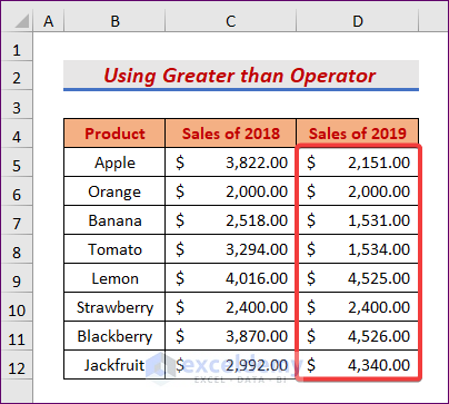
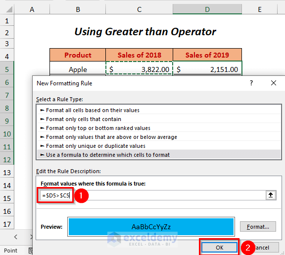
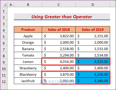
Method 3 – Conditional Formatting Based on Another Cell Range with a Greater than Operator

We will highlight the cells of the Sales of 2019 column which will be Greater than the corresponding cell ranges of the Sales of 2018 column.

Step 1:

• Follow Step 1 of Method 1. You will get the following New Formatting Rule dialog box.

• Use the following formula in the Format values where this formula is true box:

When the cells of Column D are Greater than the corresponding cells of Column C, then the Conditional Formatting will appear in that cell of Column D.

• Press OK.

Result:

Read more: Excel Highlight Cell If Value Greater Than Another Cell

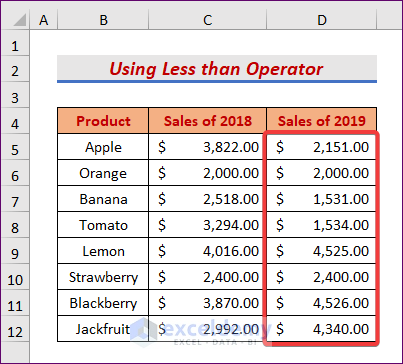
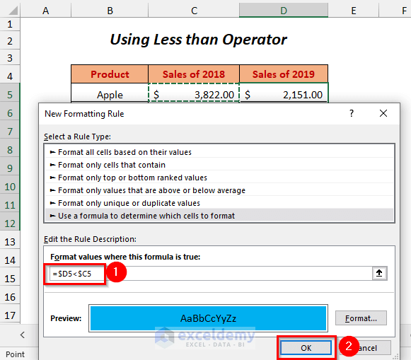
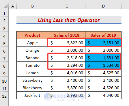
Method 4 – Using the Less than Operator for Conditional Formatting Based on Another Cell Range

You can apply Conditional Formatting to the cells of the Sales of 2019 column by using Less than Operator.

Step 1:

• Follow Step 1 of Method 1. You will get the following New Formatting Rule dialog box.

• Use the following formula in the Format values where this formula is true: Box

When the cells of Column D have a value Less than the corresponding cells of Column C, then the Conditional Formatting will appear in that cell of Column D.

• Press OK.

Result:

Read more: How to Compare Two Columns Using Conditional Formatting in Excel

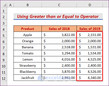
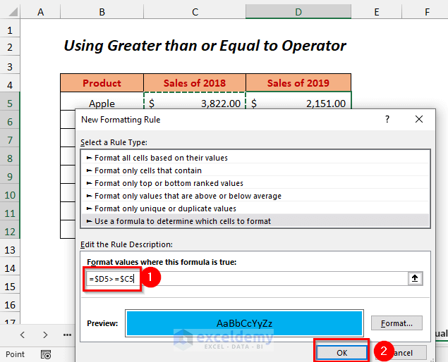
Method 5 – Conditional Formatting Based on Another Cell Range with the Greater than Or Equal to Operator

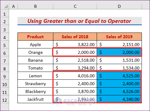
We will highlight the cells of the Sales of 2019 column which are Greater than or Equal to the corresponding cell ranges of the Sales of 2018 column.

Step 1:

• Follow Step 1 of Method 1. You will get the following New Formatting Rule Dialog Box.

• Use the following formula in the Format values where this formula is true box.

When the cells of Column D are Greater than or Equal to the corresponding cells of Column C, then the Conditional Formatting will appear in that cell of Column D.

• Press OK.

Result:

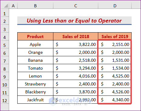
Method 6 – Using the Less than Or Equal to Operator for Conditional Formatting Based on Another Cell Range

You can apply Conditional Formatting to the cells of the Sales of 2019 column by using Less than or Equal to Operator.

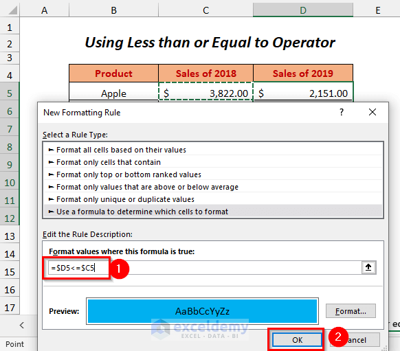
Step 1:

• Follow Step 1 of Method 1. You will get the following New Formatting Rule Dialog Box.

• Use the following formula in the Format values where this formula is true box:

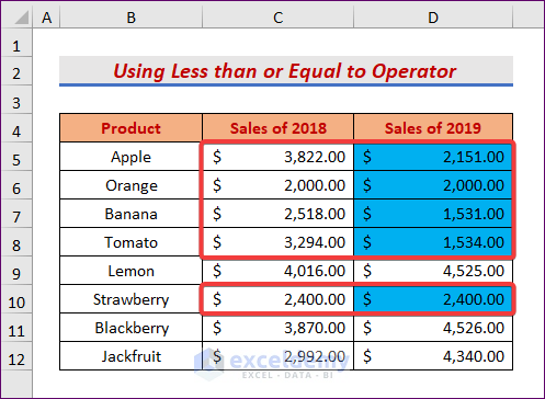
When the cells of Column D are Less than or Equal to the corresponding cells of Column C, then the Conditional Formatting will appear in that cell of Column D.

• Press OK.

Result:

Method 7 – Conditional Formatting for Multiple Conditions Using the AND Function

We want to highlight the cells of the Sales of 2019 column whose values are greater than the corresponding values of the cells of the Sales of 2018 column and the Sales of 2020 column.

Steps:

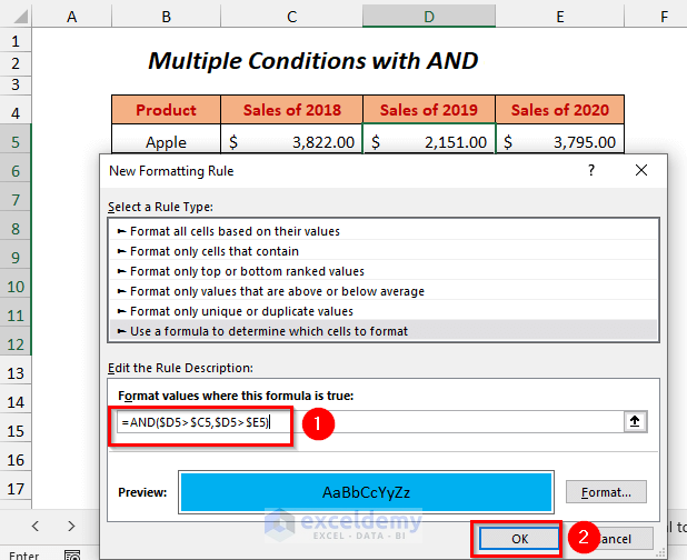
• Follow Step 1 of Method 1. You will get the following New Formatting Rule Dialog Box.

• Use the following formula in the Format values where this formula is true: Box

When the cells of Column D are Greater than the corresponding cells of Column C and Column E, then the Conditional Formatting will appear in that cell of Column D.

• Press OK.

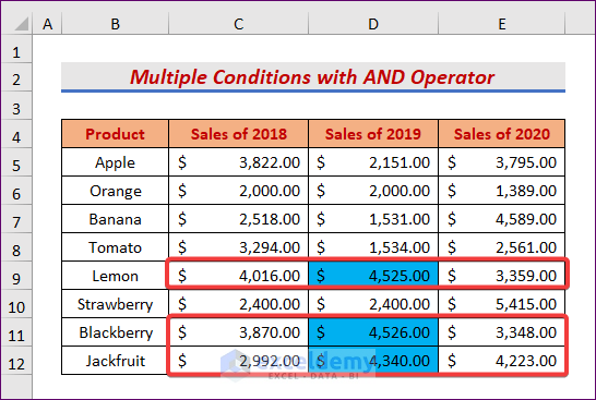
Result:

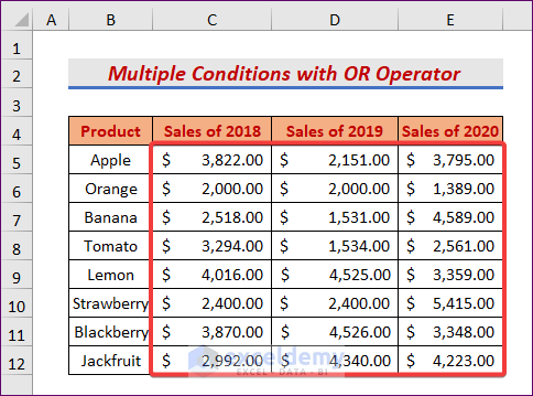
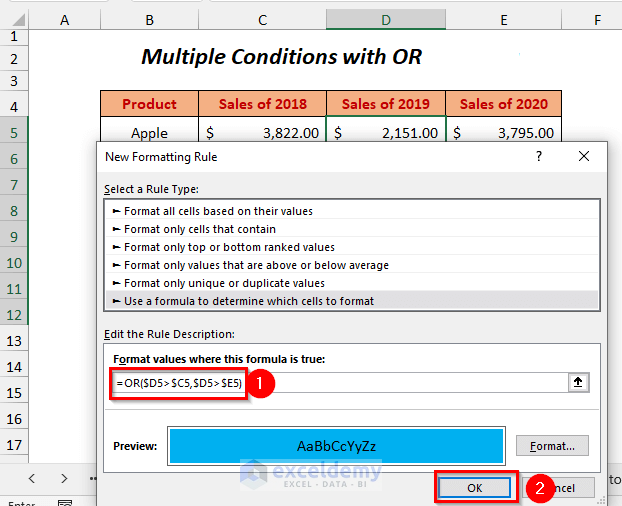
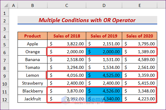
Method 8 – Conditional Formatting for Multiple Conditions Using the OR Function

We’ll highlight the cells of the Sales of 2019 column whose values are greater than the corresponding values of the cells of the Sales of 2018 column or the Sales of 2020 column.

Steps:

• Follow Step 1 of Method 1. You will get the following New Formatting Rule Dialog Box.

• Use the following formula in the Format values where this formula is true box:

When the cells of Column D are Greater than the corresponding cells of Column C or Column E, the Conditional Formatting will appear in that cell of Column D.

• Press OK.

Result:

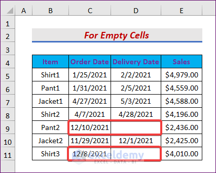
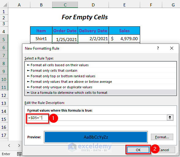
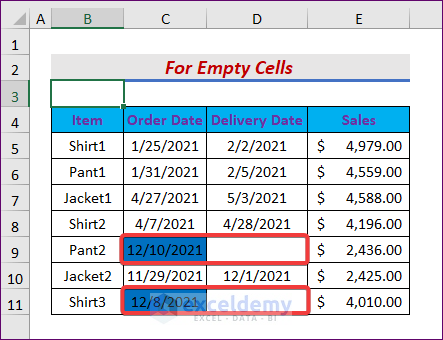
Method 9 – Conditional Formatting Based on Another Cell Range for Empty Cells

We want to highlight the Order Dates corresponding to the Delivery Dates which are empty.

Step 1:

• Follow Step 1 of Method 1. You will get the following New Formatting Rule Dialog Box (We have changed the Background Color and selected the Order Date column for Conditional Formatting).

• Use the following formula in the Format values where this formula is true box:

When the cells of Column D are Equal to Blank, the Conditional Formatting will appear to the corresponding cells of Column C.

• Press OK.

Result:

Read More: How to Apply Conditional Formatting for Blank Cells in Excel

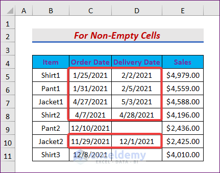
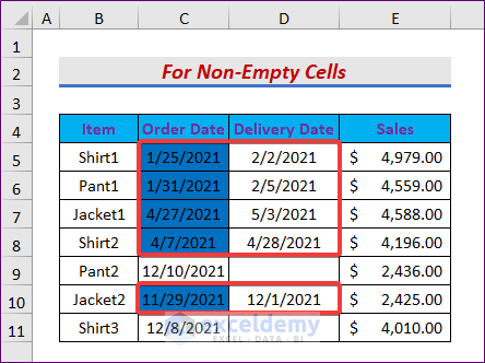
Method 10 – Conditional Formatting Based On Another Cell Range for Non-Empty Cells

We’ll highlight the Order Dates corresponding to the Delivery Dates which are non-empty.

Steps:

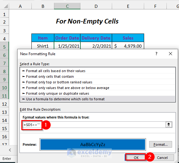
• Follow Step 1 of Method 1. You will get the following New Formatting Rule Dialog Box.

• Use the following formula in the Format values where this formula is true box:

When the cells of Column D are Not Equal to Blank, the Conditional Formatting will appear to the corresponding cells of Column C.

• Press OK.

Result:

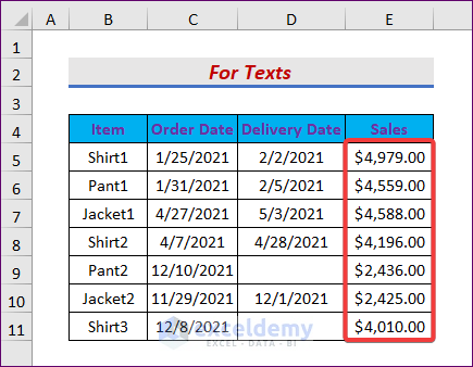
Method 11 – Conditional Formatting Based on Another Cell Range for Texts

We’ll highlight the cells of the Sales column for Jacket2 (or any other item name) in the Item column.

Steps:

• Follow Step 1 of Method 1 (We have selected the Sales column for Conditional Formatting).
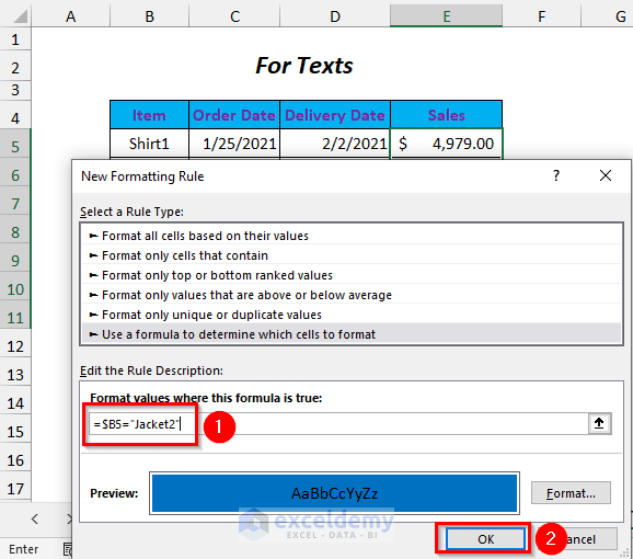
• You will get the following New Formatting Rule Dialog Box.

• Use the following formula in the Format values where this formula is true box:

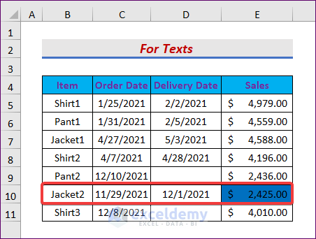
When the cells of Column B are Equal to “Jacket2”, the Conditional Formatting will appear to the corresponding cells of Column E.

• Press OK.

Result:

Read more: Excel Conditional Formatting with Formula If Cell Contains Text

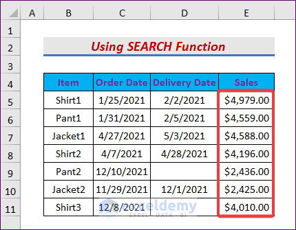
Method 12 – Conditional Formatting Using the SEARCH Function for Texts

We’ll use a partial match Jacket in the Item column to highlight the corresponding cells in the Sales column.

Steps:

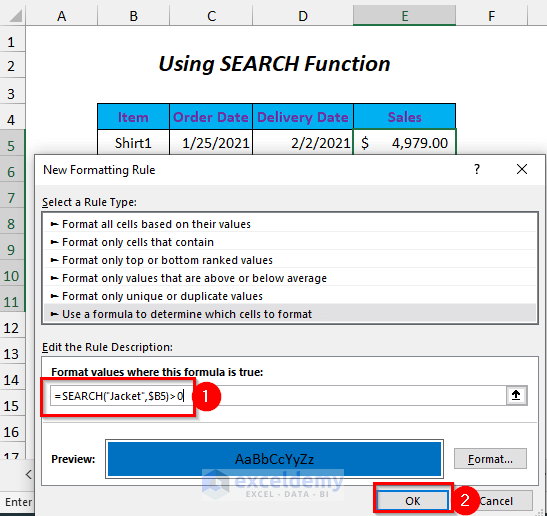
• Follow Step 1 of Method 1. You will get the following New Formatting Rule Dialog Box.

• Use the following formula in the Format values where this formula is true box:

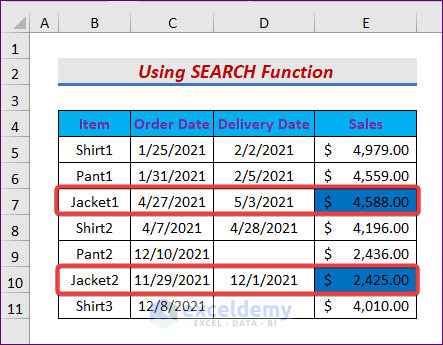
When the cells of Column B contain “Jacket”, the Conditional Formatting will appear to the corresponding cells of Column E.

• Press OK.

Result:

Download the Workbook

Further Readings

• VBA Conditional Formatting Based on Another Cell Value in Excel
• Change Font Color Based on Value of Another Cell in Excel
• How to Apply Conditional Formatting to the Selected Cells in Excel

<< Go Back to Conditional Formatting with Multiple Conditions | Conditional Formatting | Learn Excel