How to Do Conditional Formatting Based on Another Cell in Excel (6 Easy Ways)

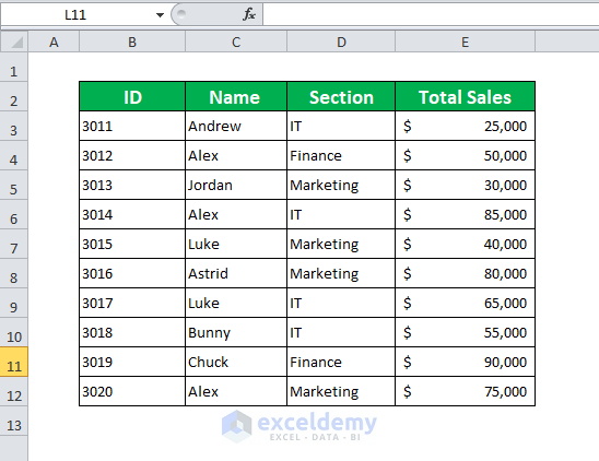
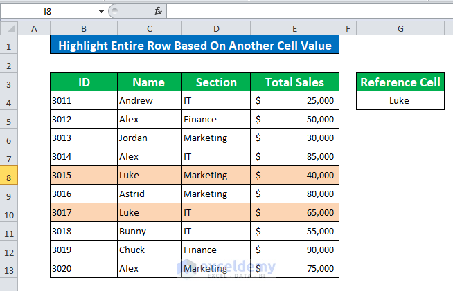
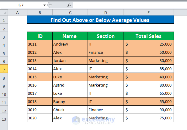
Below is a database containing the ID, Name, Section, and Total Sales of some Sales Representatives. We will format some cells using conditional formatting based on their names, sections, or total sales.

Method 1 – Highlight the Entire Row Based on Another Cell Value

Steps:

• Select the entire dataset.
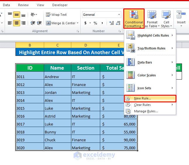
• In your Home Tab, go to Conditional Formatting in Style Ribbon.
• Click on it to open the available options
• Click on New Rule. Home → Conditional Formatting → New Rule

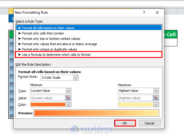
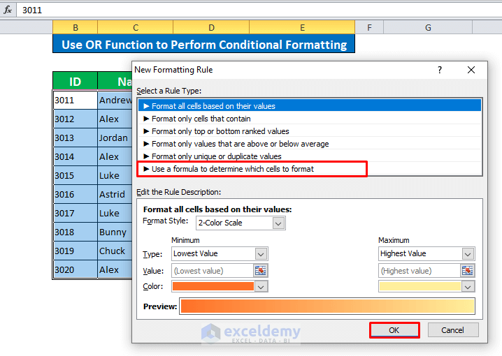
• A new window opens.
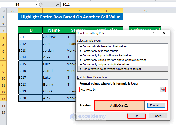
• Select Use a Formula to Determine the Cells to Format.

• In the formula section, insert this formula:

This formula will compare the dataset cells with the name Luke (G4). When the value will match, it will highlight the cell.

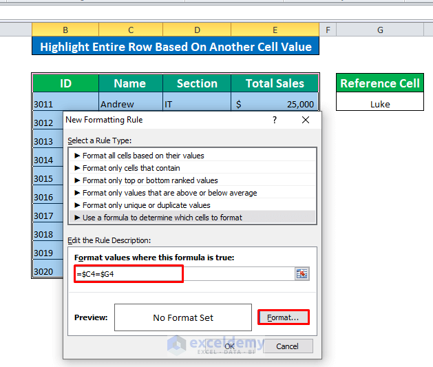
• We need to format the matched cells. The format section will help you out. We have chosen the color of the text automatically.

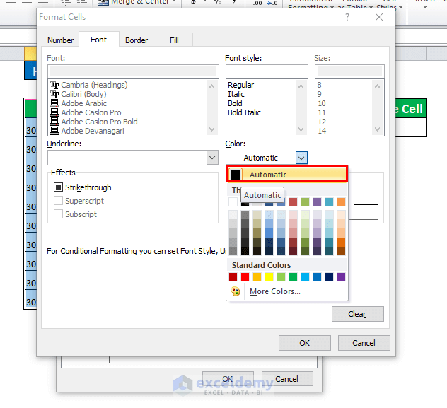
• The Fill cells option helps you highlight the cells with different colors. Choose any color you like.

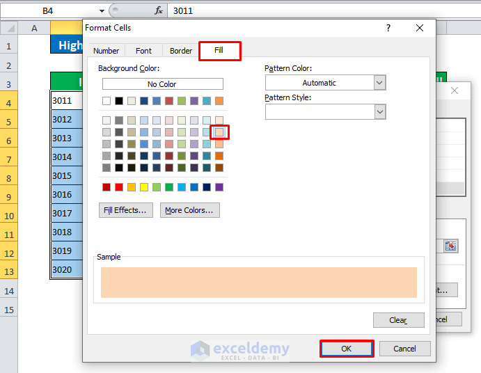
• Click OK to get the result.

Our entire rows are formatted based on the values of another cell.

Method 2 – Use the OR Function to Perform Conditional Formatting

Steps:

• Go to the New Formatting Window: Home → Conditional Formatting → New Rule

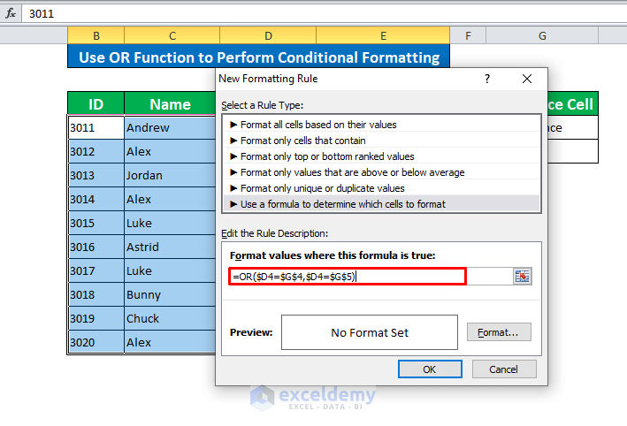
• Select Use a Formula to Determine the Cells to Format.

• Enter the OR Formula:

• Here, G4 is Finance and G5 is IT.
• The OR formula will compare the cell values with G4 and G5 and highlight the values that match the conditions.

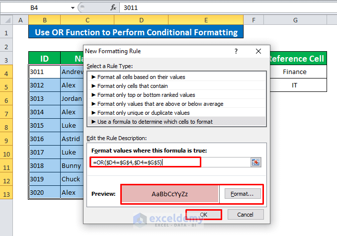
• Select a formatting style according to your preferences.
• Click OK to get the result.

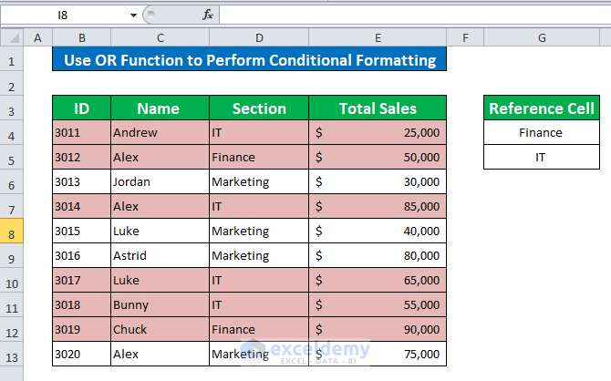
Our cells are formatted based on the reference cell values.

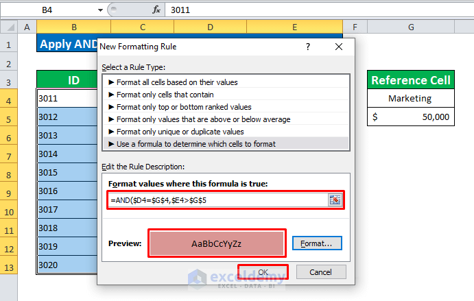
Method 3 – Apply the AND Function to Perform Conditional Formatting

Steps:

• Following the same procedures discussed above.
• Go to the New Formatting Rule window and apply the following formula:

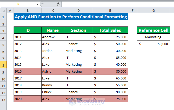
• Where G4 and G5 is Marketing and 50,000$
• Set the formatting styles and click OK to format the cells.

The cells are now formatted according to the conditions.

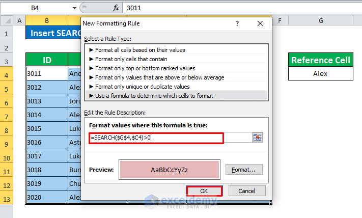
Method 4 – Insert the SEARCH Function to Perform Conditional Formatting

Steps:

• Apply the SEARCH function to find Alex. The formula is:

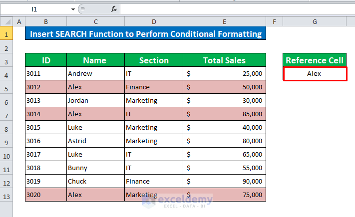
• Click OK to continue.

We have highlighted the cells that contain the name Alex.

Method 5 – Identify Empty and Non-Empty Cells Using Conditional Formatting

Steps:

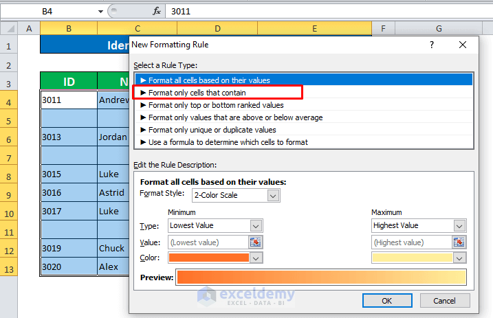
• Open the New Formatting Rule window and select Format Only the Cells that Contain.

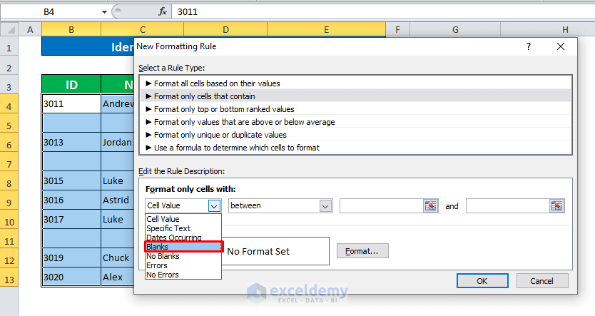
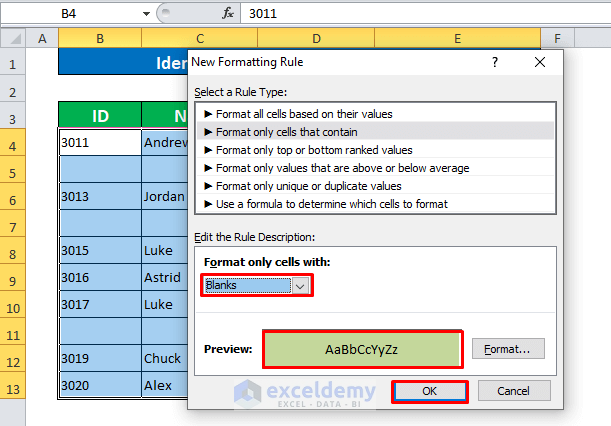
• Select Blank from the options.

• Set the Formatting and click OK to continue.

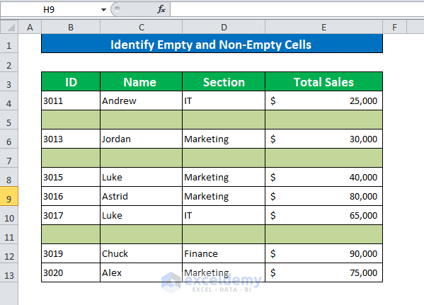
The blank cells are now identified.

Method 6 – Find the Above or Below Average Values Applying Conditional Formatting

Steps:

• To find above or below-average values, apply this formula:

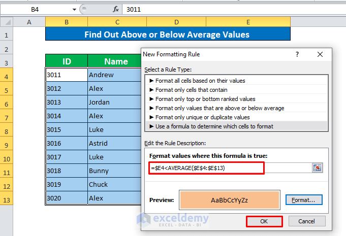
• Click OK to get the result. That’s how you can find below or above-average values.

Quick Notes

•  Once the formatting is applied, you can clear the rules.
•  We used the Absolute Cell references ($) to block the cells for the perfect result.
• When you want to find a sensitive name, you can use the FIND function instead of the SEARCH function.

Download the Practice Workbook

Download this book to practice the task.

You May Also Like to Read

• VBA Conditional Formatting Based on Another Cell Value in Excel
  
• Change Font Color Based on Value of Another Cell in Excel
• How to Apply Conditional Formatting to the Selected Cells in Excel
• Conditional Formatting Based on Multiple Values of Another Cell
• Conditional Formatting Based On Another Cell Range in Excel

<< Go Back to Conditional Formatting with Multiple Conditions | Conditional Formatting | Learn Excel