How to Apply Conditional Formatting to the Selected Cells in Excel

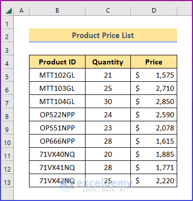
We will be using a Product Price List dataset to demonstrate applying conditional formatting in Excel.

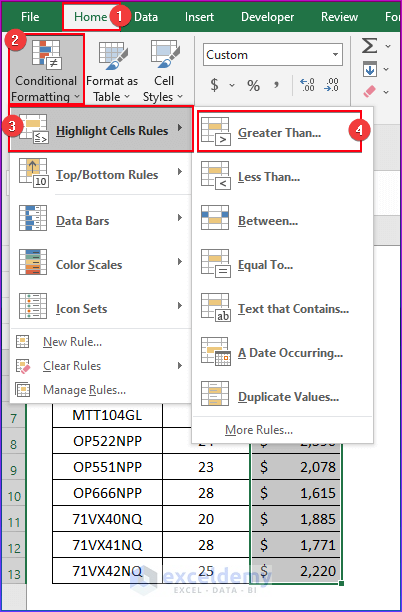
Method 1 – Using Highlight Cells Rules to Apply Conditional Formatting to the Selected Cells in Excel

Steps:

• Select the cells where you want to apply formatting, such as the price column.

• Go to Home, select Conditional Formatting, and choose Highlight Cells Rules.
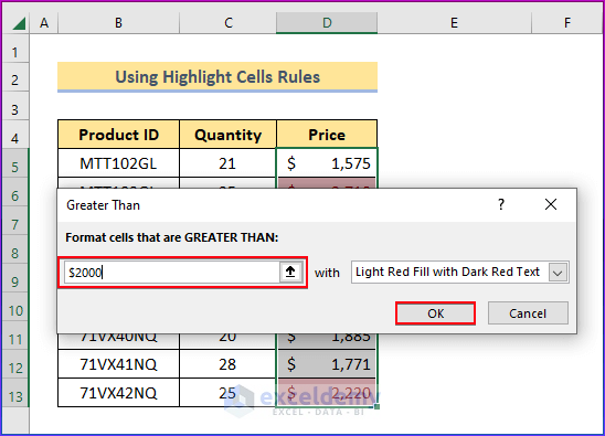
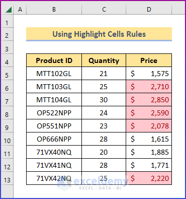
• You can use any of the commands from the list as per your requirement. For example, Greater Than command will highlight all the values greater than a value that you set as a criterion. If you select Greater Than from the list, a dialog box will appear.

• Insert $2000 within the box.
• Hit Ok.
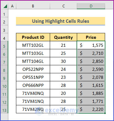
• This will highlight all the cells containing values greater than $2000:

• You will get the following output.

The other available options include:

1. Less Than
   Highlights all the cells that contain values less than an inserted value.

2. Between
   Highlights all the cells that contain values in between two inserted values.

3. Equal To
   Highlights all the cells that contain values equal to an inserted value.

4. Text that Contains
   Highlights all the cells that match the inserted text within the dialog box.

6. A Date Occurring
   Highlights records that occur on a specific date.
7. Duplicate Values
   Highlights all the cells that contain duplicate values.

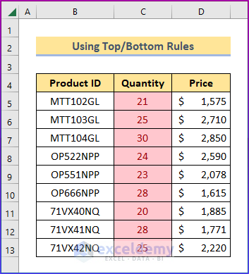
Method 2 – Using Top/Bottom Rules to Apply Conditional Formatting to the Selected Cells

Steps:

• Choose a range of cells.

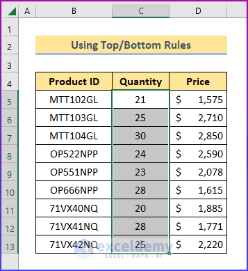
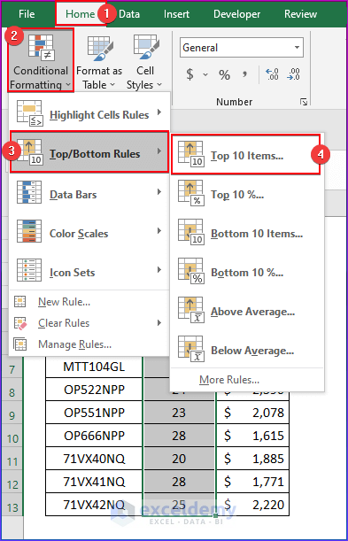
• Go to Home, select Conditional Formatting, and choose Top/Bottom Rules.
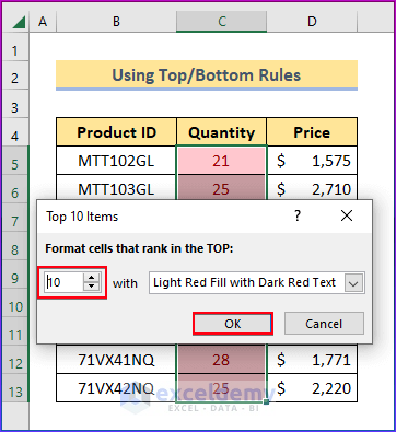
• Choose the Top 10 Items option.

• You will see a dialog box. Press OK.

• The Top 10 Items command will highlight the first 10 items from the select cells as follows.

Other options include:

1. Top 10%
   This command will highlight the first 10% of items from the range of selected cells.

2. Bottom 10 Items
   It will highlight 10 items from the bottom side of the selected range of cells.

3. Bottom 10%
   This command will highlight 10% of cells with colors from the bottom of the selected cells.

5. Above Average
   This highlights all the cells containing values above the average.
6. Below Average
   This highlights all the cells containing values below the average.

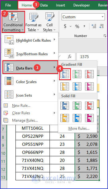
Method 3 – Using Data Bars to Apply Excel Conditional Formatting to the Selected Cells

• Select the range of cells first.
• Go to Home, select Conditional Formatting, and choose Data Bars.
• You will find two options: Gradient Fill, and Solid Fill. Both options offer bars with a variety of colors.

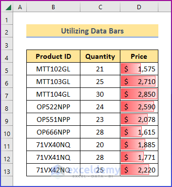
• If you select Gradient Fill, it will highlight cells with a gradient color as in the following picture. The bars automatically scale based on the maximum value found within the range and start from 0.

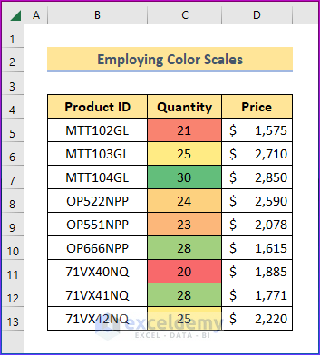
Method 4 – Inserting Color Scales to Conditionally Format the Selected Cells in Excel

• Select the cell range.
• Navigate to Home, then select Conditional Formatting and choose Color Scales.
• Select a scale such as Green-Yellow-Red Color Scale.

• This color scale applies green to the largest values, yellow to the middle values, and red to the lowest.

Method 5 – Using Icon Sets to Apply Excel Conditional Formatting to the Selected Cells

• Select the range of cells.
• Go to Home, then to Conditional Formatting, and select Icon Sets.
• You will see a list of options.

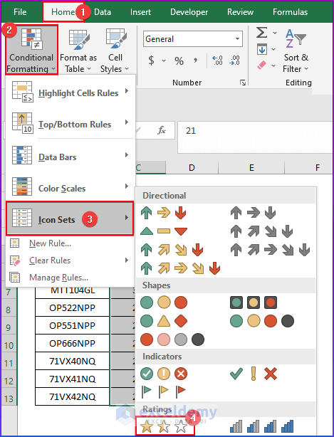
There are different types of icons under 4 categories:

1. Directional
2. Shapes
3. Indicators
4. Ratings

• If we choose to start from the Rating category, we will see the result like the picture below.

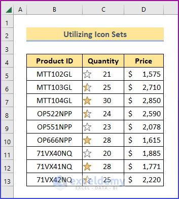
• The highest quantity is marked with a full star, the lowest with an empty star, and the in-betweens with a half-filled star.

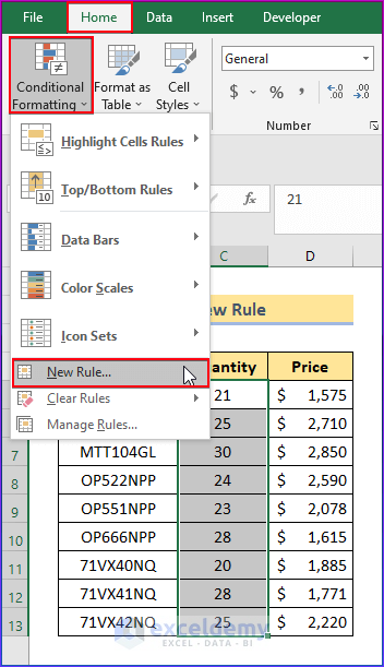
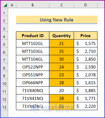
Method 6 – Applying a New Rule to Conditionally Format the Selected Cells

• Select the range of cells.
• Go to Home, then to Conditional Formatting, and select New Rule.

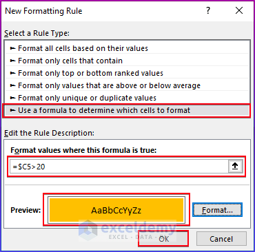
• If you select Use a formula to determine which cells to format, you will get to the box to insert the formula.
• Insert the formula below to highlight all the cells with values greater than 20 in the quantity column.

• Hit the OK button.

• Here’s the result.

Download the Practice Workbook

Related Articles

• VBA Conditional Formatting Based on Another Cell Value in Excel
• How to Do Conditional Formatting Based on Another Cell in Excel
• Change Font Color Based on Value of Another Cell in Excel
• Conditional Formatting Based on Multiple Values of Another Cell
• Conditional Formatting Based On Another Cell Range in Excel

<< Go Back to Conditional Formatting | Learn Excel