Data Bars in Excel (Insert, Format, and Deal with Negative Values)

This is an overview:

Download Practice Workbook

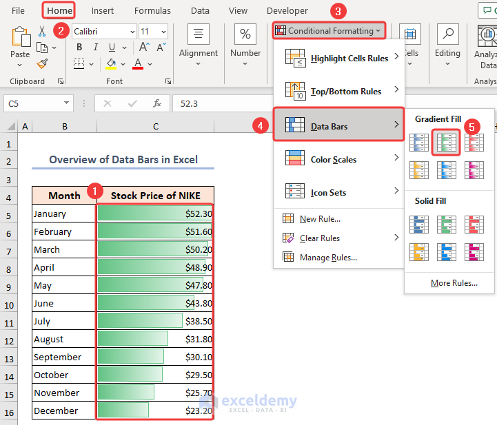
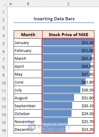
How to Insert Data Bars in Excel?

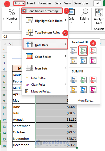
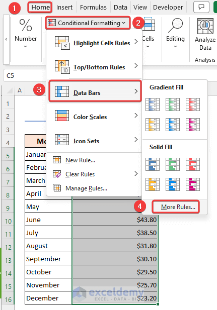
• Select data and choose a Gradient Fill: go to Home>>Conditional Formatting>>Data Bars.

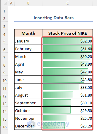
• Data bars will be inserted for the selected data.

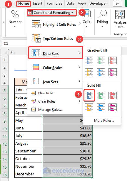
• You can also choose solid fill: choose a color in Solid Fill (Home>>Conditional Formatting>>Data Bars).

This is the output.

How to Format Data Bars in Excel?

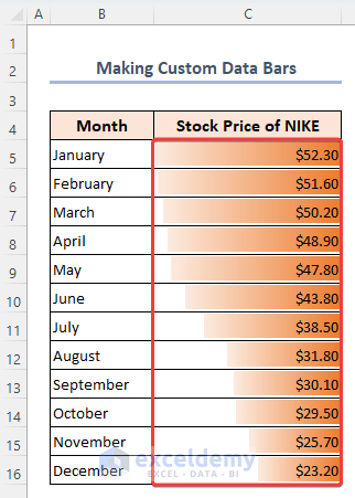
1. Creating Custom Data Bars

• In the Home tab, open Conditional Formatting.
• Choose More Rules in Data Bars.

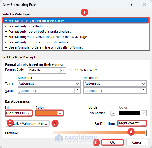
• In the New Formatting Rule window, choose Format all cells based on their values.
• Customize the data bars. Here, Gradient Fill was chosen in Fill.
• Change the Color and Direction , as shown below and click OK.

This is the output.

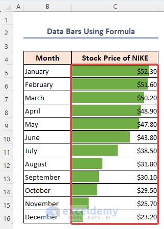
2.  Format Data Bars Using a Formula

• Go to More Rules in Conditional Formatting.
• in New Formatting Rule click Format all cells based on their values.
• Change the type to Formula.
• Enter the formula (with the MIN and MAX functions), and click OK.

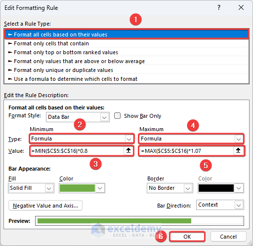
This is the output.

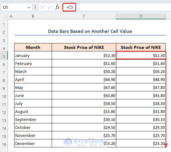
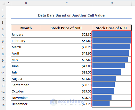
 Format Data Bars Based on Another Cell Value

• Select D5 and enter the formula;
• Drag down the Fill Handle to see the result in the rest of the cells.

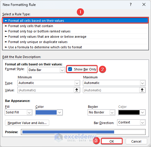
• Go to New Formatting Rule and choose Format all cells based on their values.
• Check Show Bar Only and click OK.

This is the output.

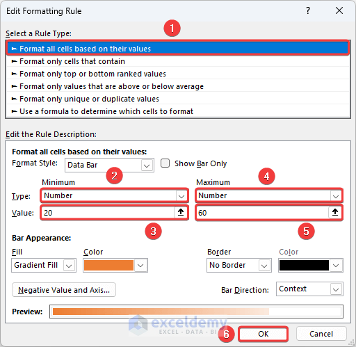
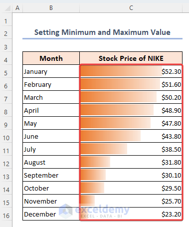
4. Format data bars Setting the Minimum and Maximum Value

• Open the New Formatting Rule window and select Format all cells based on their values.
• Choose Number.
• Enter minimum and maximum values and click OK.

This is the output

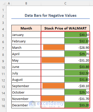
5. Format Data Bars with Negative Values

The dataset showcases WALMART stock prices in different Months. There are negative prices.

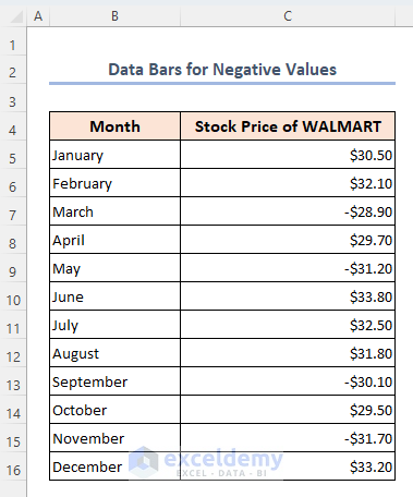
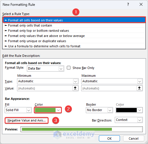
• Open the New Formatting Rule window and choose Format all cells based on their values.
• Choose a color for the positive values and select Negative Value and Axis options.

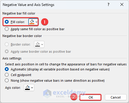
• Choose a Fill color for negative values and click OK.

This is the output

Which Things to Remember While Using Data Bars in Excel?

• You can also change the data bars orientation to vertical position.

Frequently Asked Questions

1. How do I remove data bars from a cell or range in Excel?

Answer: Go to the Home tab, click Conditional Formatting, and choose Clear Rules.

2. What types of data can be represented using data bars in Excel?

Answer: Data bars can represent numerical data: values, percentages or other numerical inputs with formulas.

3. How do I adjust the width or length of data bars in Excel?

Answer: Select the cells or range with data bars and go to the Home tab. Select Conditional Formatting and choose Manage Rules.

Data Bars in Excel: Knowledge Hub

• Add Data Bars
• Use Data Bars with Percentage
• Define Maximum Data Bars Value
• Add Solid Fill Data Bars
• Conditional Formatting Data Bars Different Colors
• Conditional Formatting with Data Bars Based on Another Cell
• [Fixed]: Conditional Formatting in Data Bar Percentage Not Working

<< Go Back to Conditional Formatting | Learn Excel