In Microsoft Excel, there is a feature named Conditional Formatting that allows you to apply formatting to cells based on certain criteria. We can use Conditional Formatting with data bars based on the value of another cell. In this article, I am going to explain the whole procedure of how to use Conditional Formatting data bars based on another cell in Excel.
How to Use Conditional Formatting with Data Bars Based on Another Cell in Excel: Step-by-Step Procedures
We can divide the whole process of how to use Conditional Formatting data bars based on another cell in Excel into three different steps.
Step 1: Create an Organised Dataset
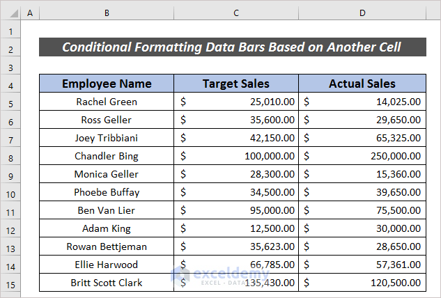
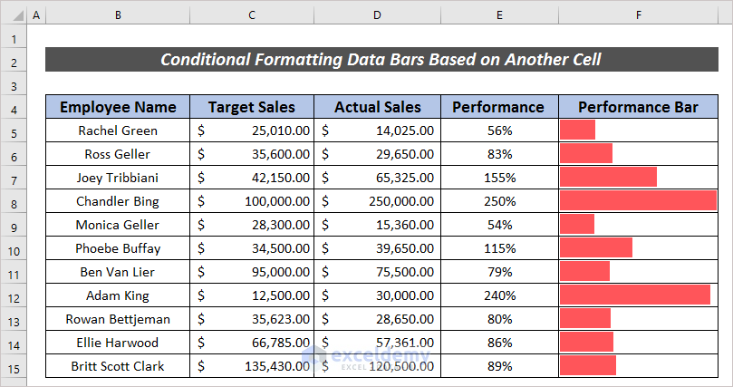
We often use the Conditional Formatting feature based on a certain criterion. For this, we need an organized dataset where we can apply a certain condition. I have the information on a company’s sales. I want to visualize their performance with data bars based on another cell.
Steps:
- Select a cell and apply the following formula to improve the work efficiency of employees.
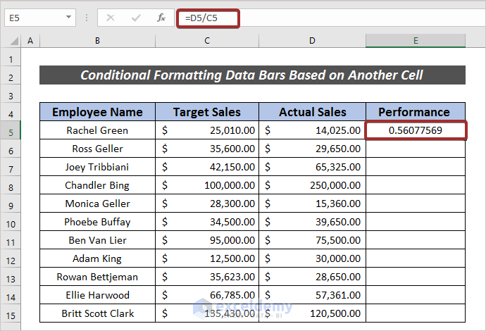
=D5/C5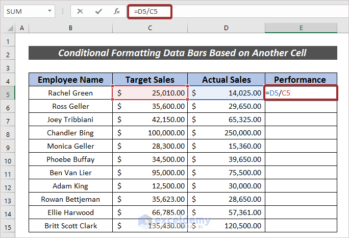
- Press ENTER to have the output.
- To convert it into a percentage, click on Percentage Sign from the ribbon under the Home tab.
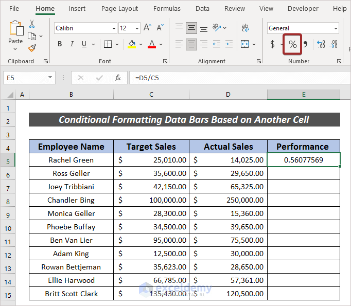
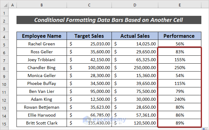
Thus, we will have the value in the percentage form.
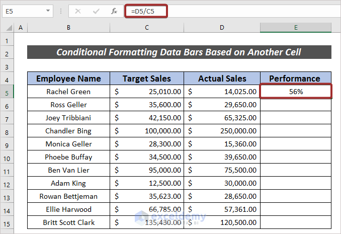
- Afterward, use Fill Handle to AutoFill the rest cells.
Step 2: Use Formula to Link a Cell with Another One
Linking a cell to another cell is also a part of this process. To accomplish it, follow the following steps.
Steps:
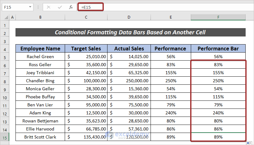
- Pick a cell (i.e. F5) and input the following formula there.
=E5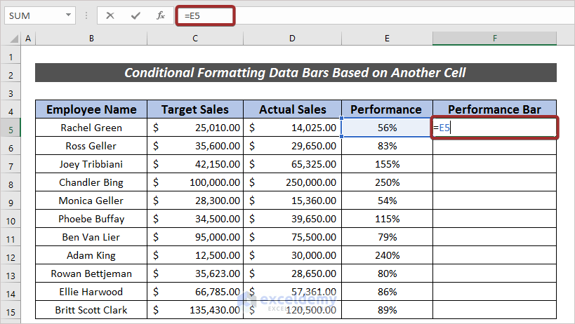
- Followingly, press ENTER.
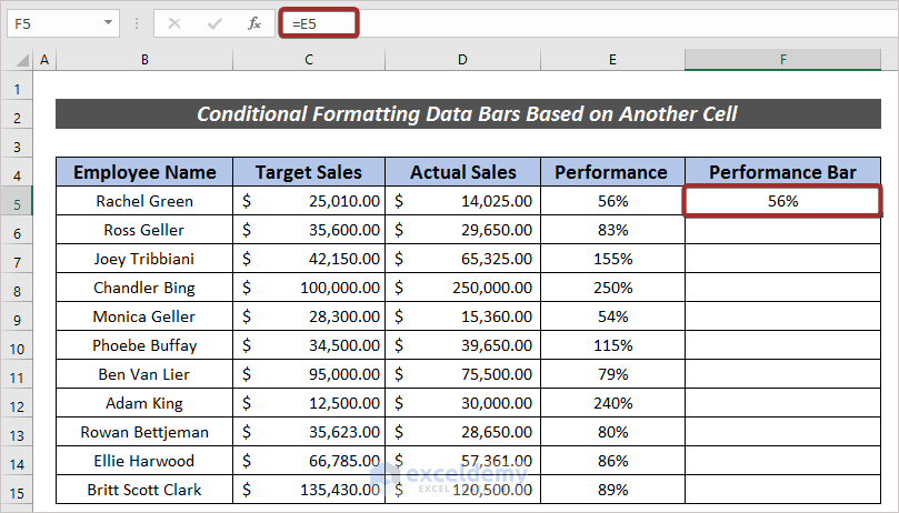
- AutoFill the remaining cells.
Step 3: Apply Conditional Formatting with Data Bars
After having a complete dataset, we can now apply a condition and display the results with data bars through the Conditional Formatting feature.
Steps:
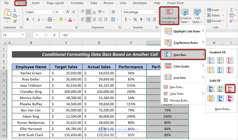
- Select the related cells first (i.e. F5:F15) and go to Home.
- Next, click on Conditional Formatting from the ribbon and choose Data Bars.
- After that, pick a color from the Solid Fill group.
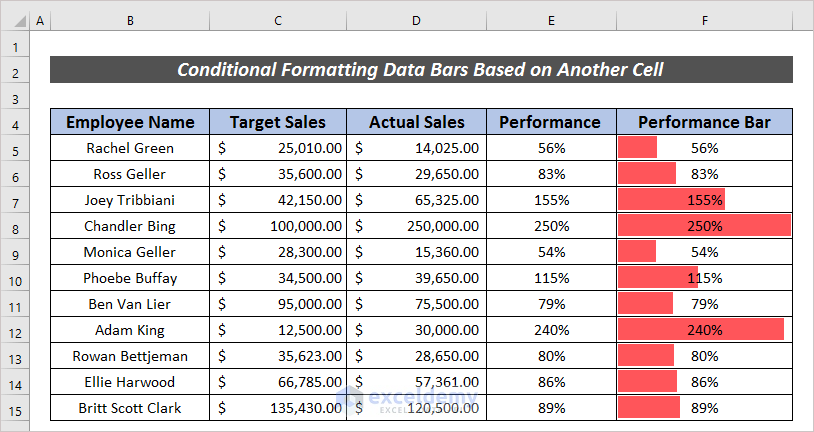
- Now, we will have the data bar with efficiency values.
- You can also show their performance value with only data bars. For this-
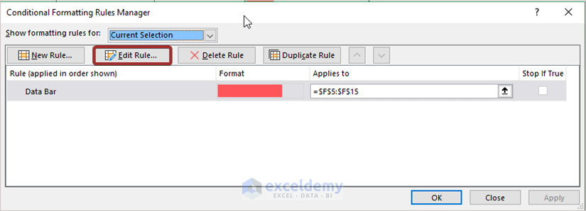
- Click on Manage Rules… from the Conditional Formatting option.
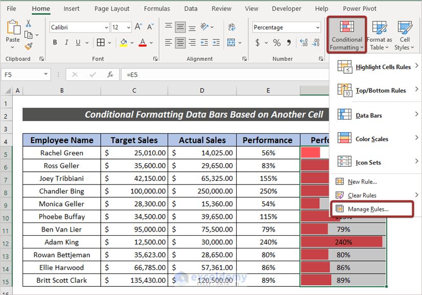
- Then, click on Edit Rule.
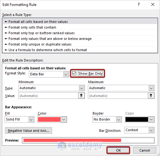
- Followingly, check the Show Bar Only option.
- Then, press OK.
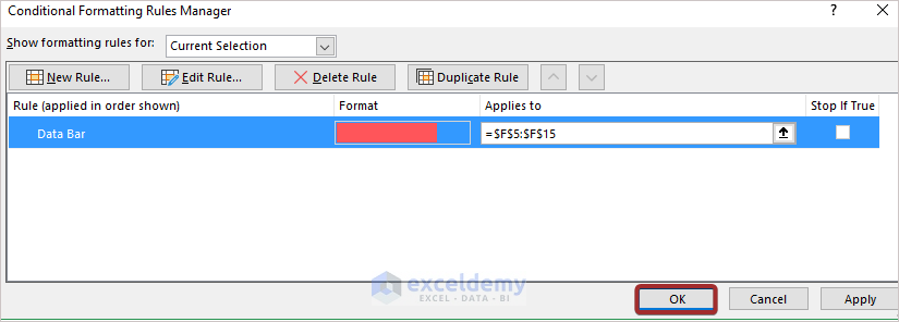
- Press OK from the Conditional Formatting Rules Manager wizard.
- Thus, we will have Conditional Formatting data bars based on another cell in Excel.
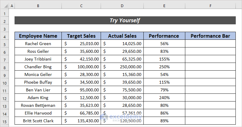
Practice Section
For more expertise, you can practice here.
Download Practice Workbook
Conclusion
At the end of this article, I like to add that I have tried to explain the whole procedure of how to use Conditional Formatting data bars based on another cell in Excel. It will be a matter of great pleasure for me if this article could help any Excel user even a little. For any further queries, comment below. You can visit our site for more articles about using Excel.
Related Articles
- How to Add Data Bars in Excel
- How to Add Solid Fill Data Bars in Excel
- How to Add Blue Data Bar in Excel
- How to Use Data Bars with Percentage in Excel
- How to Define Maximum Data Bars Value in Excel
- How to Remove Data Bars in Excel
- [Solved]: Data Bars Not Working in Excel
- Conditional Formatting Data Bars Different Colors
- [Fixed]: Conditional Formatting in Data Bar Percentage Not Working in Excel
<< Go Back to Data Bars | Conditional Formatting | Learn Excel
Get FREE Advanced Excel Exercises with Solutions!
