Excel is the most widely used tool when it comes to dealing with huge datasets. We can perform myriads of tasks of multiple dimensions in Excel. Sometimes, while working in Excel, we need to take the help of data bars. However, some problems may arise in data bars. In this article, I will cover 3 such cases of data bars in Excel not working.
Data Bars Not Working in Excel: 3 Causes and Solutions
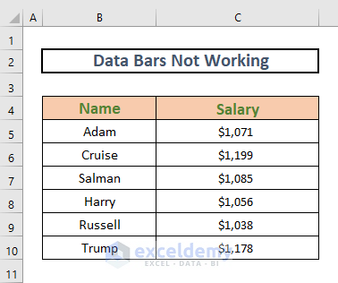
This is the dataset for today’s article. I have some employees along with their salaries. I will use data bars to depict the salaries.
1. Avoid Non-Numerical Value
The first case of the data bar not working might be that the cell values are non-numeric. When you select non-numeric data such as name, and address, and apply a data bar, it will not work. Let’s see it step by step.
Steps:
- Select a non-numeric data range. I am going to select B5:B10.
- Then go to the Home tab >> Conditional Formatting >> Data Bars >> Choose any fill.

- You will see that Excel has not applied any data bar.
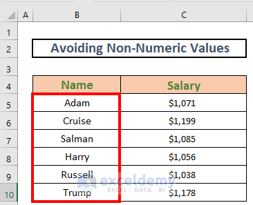
Reason: As I have mentioned earlier, data bars are not applicable for non-numeric values. Since the Name is not numeric, Excel will not apply data bars.
Solution: Avoid non-numerical values when applying data bars.
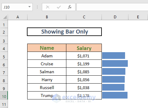
2. Show Data and Bar Separately
When you apply a data bar, the fill color and text color combination may not get along with each other well, and hence the dataset does not look visually appealing. See the image below as an example.
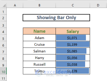
You can get rid of this problem if you show only the data bars in a separate column. Let’s see how to do so.
Steps:
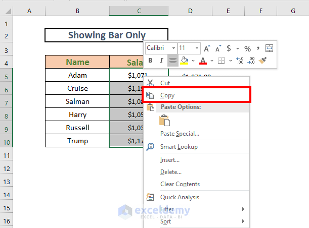
- Copy C5:C10 using the context menu.
- Then, paste them into D5:D10.
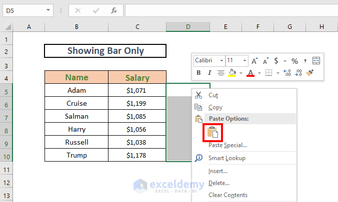
- Excel will paste them in D5:D10.
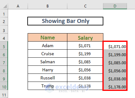
- Then go to the Home tab >> Conditional Formatting >> Data Bars >> Choose any fill.

- Excel will apply data bars.
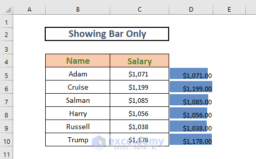
- Now, go to Conditional Formatting >> Manage Rules.

- A box named Conditional Formatting Rules Manager will pop up. Select Edit Rule.
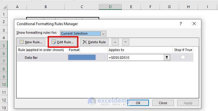
- Edit Formatting Rule box will appear. Check the Show Bar Only Then press OK.

- You will see that Excel has applied data bars in a separate column and the dataset is looking neater.
Read More: How to Add Solid Fill Data Bars in Excel
3. Set a Minimum Value Manually
Now, I will discuss another problem of working with data bars. When you are dealing with large numbers and the differences among these numbers are very small, data bars do not depict the difference well. See the image below for a better understanding. Here, I have the Months and the amount of Sales in those months.
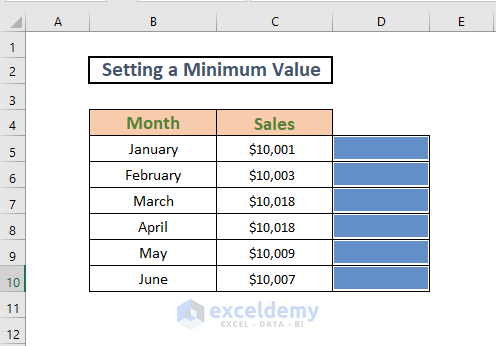
Since the differences between the numbers are very small, the bars are showing no differences. We can deal with the problem following this procedure.
Steps:
- Bring the Edit Formatting Rule box following the previous section.
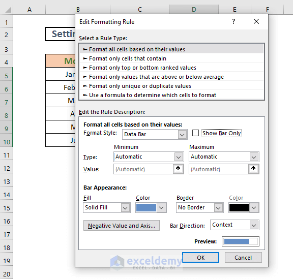
- Then choose the type as Number and set the value 10000 under the Minimum Then click OK.

- Now you will see the clear differences among the numbers.
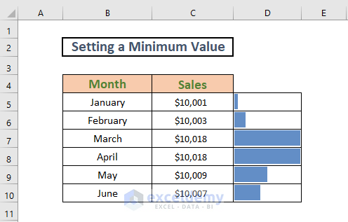
Explanation: Excel is now depicting the numbers considering 10000 as the origin. It increases the length by one unit when you increase the numbers by one each time keeping 10000 as the reference point.
Things to Remember
Data bars are applicable for numeric values only.
Download Practice Workbook
Download this workbook and practice while going through this article.
Conclusion
In this article, I have discussed 3 cases of data bars in Excel not working. I hope it helps everyone. If you have any kind of suggestions, ideas, or feedback, please feel free to comment down below.
Related Articles
- How to Add Data Bars in Excel
- How to Add Blue Data Bar in Excel
- How to Define Maximum Data Bars Value in Excel
- How to Remove Data Bars in Excel
- How to Use Data Bars with Percentage in Excel
- Conditional Formatting Data Bars Different Colors
- Conditional Formatting with Data Bars Based on Another Cell in Excel
- [Fixed]: Conditional Formatting in Data Bar Percentage Not Working in Excel
<< Go Back to Data Bars | Conditional Formatting | Learn Excel
Get FREE Advanced Excel Exercises with Solutions!
