While working in Microsoft Excel, it may be necessary to represent values in graphs and this is where Data Bars come in handy. In fact, they add visual depth and clarity to the information. With this purpose, this article wishes to demonstrate 2 easy methods on how to add solid fill data bars in Excel.
What Are Data Bars?
Data Bars are a feature of the Conditional Formatting tool, allowing us to insert a bar chart inside the cells. In fact, the size of the bars depends on the value of the cell. Simply put, larger values have a bigger bar line while smaller values have a small bar line. Moreover, data bars help us visualize the values of the cells at a glance.
1. Using Conditional Formatting to Add Solid Fill Data Bars in Excel
Excel’s Conditional Formatting option helps users change the looks of a dataset based on certain criteria like minimum or maximum numbers, range of values, etc.
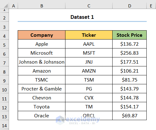
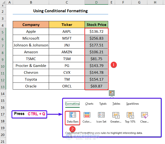
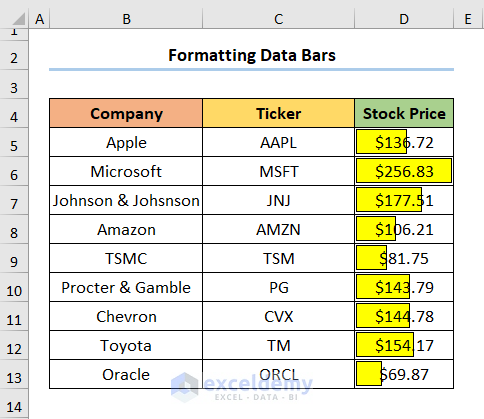
To illustrate the first method, let’s consider the dataset in the B4:D13 cells, which shows the Company names, the company Ticker, and the Stock Price in USD.
So, without further delay, let’s look at the following methods step-by-step.
📌 Steps:
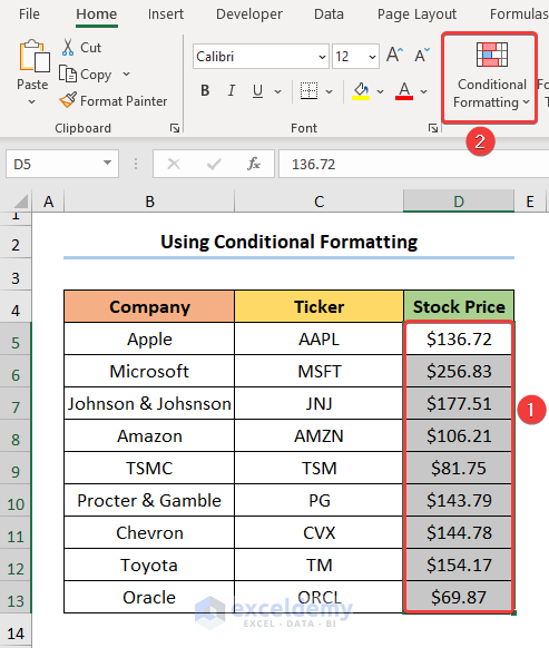
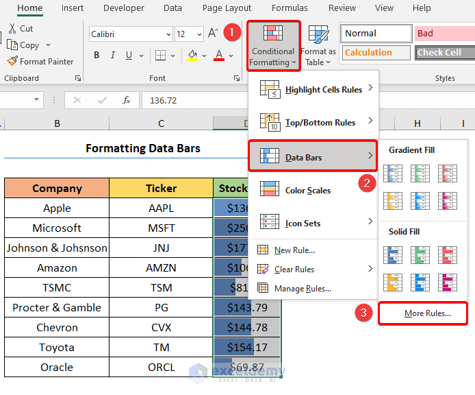
- Firstly, select the Stock Price values in the D5:D13 cells and click the Conditional Formatting drop-down.
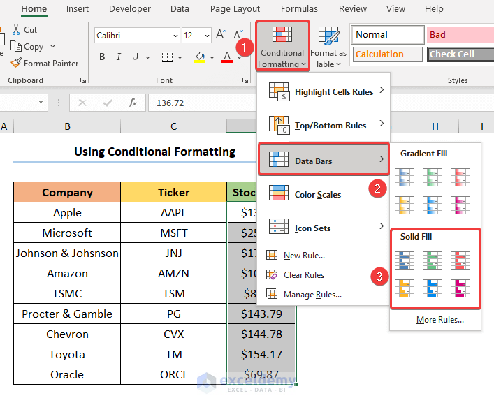
- Secondly, select Conditional Formatting > Data Bars > Solid Fill as shown in the image below.
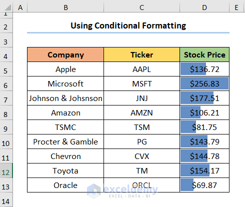
That’s it, you have successfully added Solid Fill Data Bars to your dataset.
📋 Note: You can also add Data Bars by selecting the cells and Pressing CTRL + Q to access the Quick Analysis tool.
2. Applying Solid Fill Data Bars with Excel VBA Code
Although adding Data Bars is very easy, if you need to do it often, then you may consider the VBA code below. So, just follow these steps bit by bit.
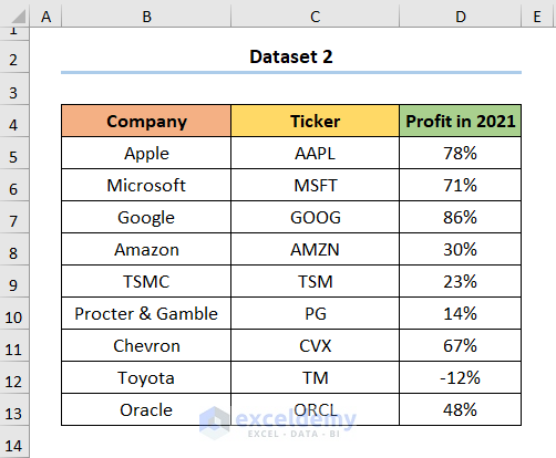
Assuming the dataset given below in the B4:D13 cells. Here, the dataset shows the Company names, the company Ticker, and the 2021 Profit in USD.
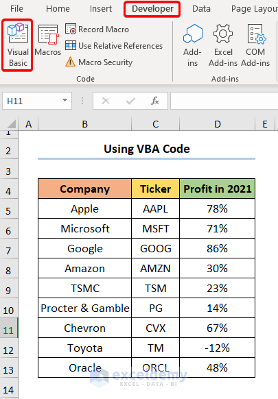
📌 Step 01: Open the Visual Basic Editor
- Firstly, go to the Developer > Visual Basic.
📌 Step 02: Insert the VBA Code
- Secondly, insert a Module where you’ll paste the VBA code.

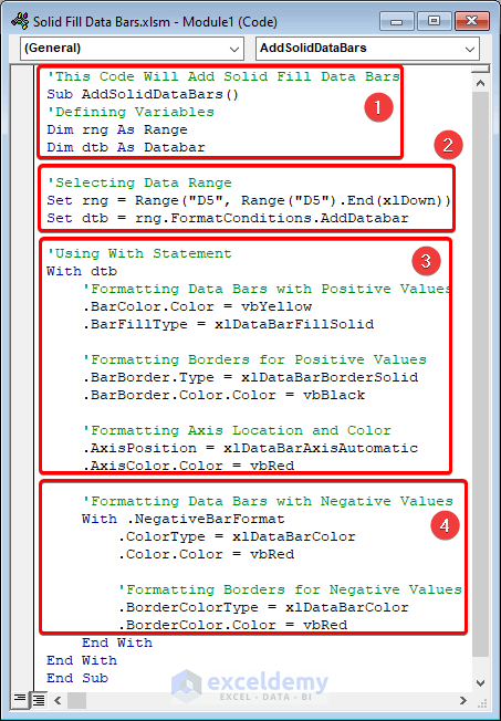
For your ease of reference, you can copy and paste the code from here.
Sub AddSolidDataBars()
Dim rng As Range
Dim dtb As Databar
Set rng = Range("D5", Range("D5").End(xlDown))
Set dtb = rng.FormatConditions.AddDatabar
With dtb
    .BarColor.Color = vbYellow
    .BarFillType = xlDataBarFillSolid
    .BarBorder.Type = xlDataBarBorderSolid
    .BarBorder.Color.Color = vbBlack
    .AxisPosition = xlDataBarAxisAutomatic
    .AxisColor.Color = vbRed
    With .NegativeBarFormat
        .ColorType = xlDataBarColor
        .Color.Color = vbRed
        .BorderColorType = xlDataBarColor
        .BorderColor.Color = vbRed
    End With
End With
End Sub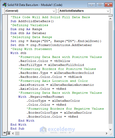
💡 Code Breakdown:
Now, I will explain the VBA code for adding Solid Fill Data Bars. In this case, the code is divided into 4 parts.
- 1- Firstly, give a name to the sub-routine, and define the variables.
- 2- Secondly, use the Set statement to select the cells and add Data Bars.
- 3- Thirdly, apply the With statement to perform tasks like adding bar color, fill type, axis position, etc. for the Solid Fill Data Bars with positive value.
- 4- Finally, nest a second With statement for formatting the Solid Fill Data Bars with negative values.
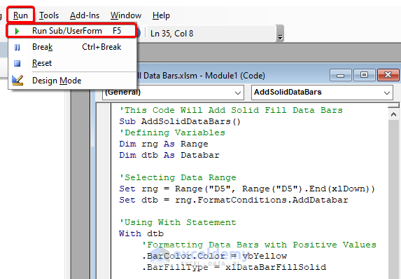
📌 Step 03: Run the VBA Code
- Thirdly, press the F5 key to run the VBA Code.
Finally, the results should look like the picture given below.

Read More: Conditional Formatting Data Bars Different Colors
How to Format Solid Fill Data Bars in Excel
Now that you’ve learned how to add the Solid Fill Data Bars, let’s see how to make changes to the default settings, to get better-looking bars. So, follow along.
- At the very beginning, select the Stock Price values and go to Conditional Formatting > Data Bars > More Rules.
Next, the New Formatting Rule wizard appears which allows you to customize the Data Bars according to your preference.
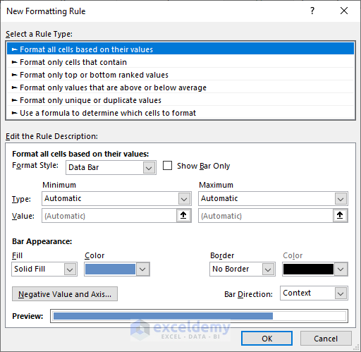
In the following section, we’ll discuss how to customize Solid Fill Data Bars.
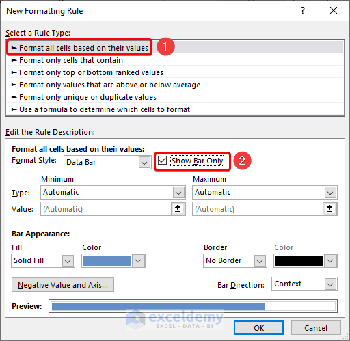
Hiding Data Values in Solid Fill Data Bars in Excel
Sometimes, you might need to hide data values while using the Solid Fill Data Bars. You can easily hide the data values from the cells in case the Data Bars look cluttered.
- Initially, choose the Format all cells based on their values, followed by the Show Bar Only option.
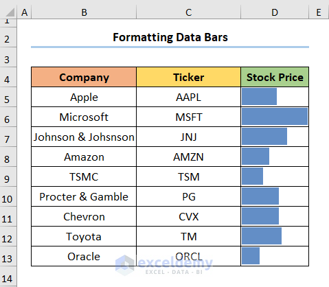
This gives the outcome as shown in the image below.
Read More: Conditional Formatting with Data Bars Based on Another Cell in Excel
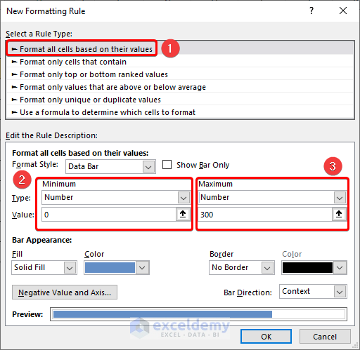
Setting Maximum and Minimum Values for Data Bar
Next, you can set the maximum and minimum values for your Solid Fill Data Bars. Now, the default option is set to Automatic but you can change it by following the steps below.
- In a similar fashion, set the Type to Number for both Minimum and Maximum groups.
- Next, set the Values as shown in the picture below.
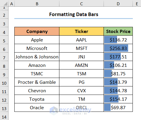
The results appear as shown below.
Read More: How to Define Maximum Data Bars Value in Excel
Changing Solid Fill Data Bar Color and Border
Lastly, you can change the color of the Solid Fill Data Bars and their border. It’s easy, just follow these simple steps.
- Similarly, navigate to the Bar Appearance group and select a suitable color.
- Then, choose the Solid Border option and set the border color to black.

The results should look like the following picture.
🔔 Things to Remember
- Firstly, Solid Fill Data Bars apply only to numeric values and not text data.
- Secondly, unlike Excel Charts, Solid Fill Data Bars only apply on the horizontal axis.
Download Practice Workbook
You can download the practice workbook from the link below.
Conclusion
I hope this article helped you understand how to add solid fill data bars in Excel. If you have any queries, please leave a comment below.
Related Articles
- How to Use Data Bars with Percentage in Excel
- [Solved]: Data Bars Not Working in Excel
- How to Add Data Bars in Excel
- How to Add Blue Data Bar in Excel
- How to Remove Data Bars in Excel
- [Fixed]: Conditional Formatting in Data Bar Percentage Not Working in Excel
<< Go Back to Data Bars | Conditional Formatting | Learn Excel
Get FREE Advanced Excel Exercises with Solutions!
