How to Add Blue Data Bar in Excel (3 Easy Ways)

We occasionally need to use the data bars feature to display our dataset. We can rapidly do it with Excel’s conditional formatting feature. In this tutorial, I’ll show you three suitable ways to add a blue data bar in Excel effectively with appropriate illustrations.

Download Practice Workbook

Download this practice workbook to exercise while you are reading this article.

3 Suitable Ways to Add Blue Data Bar in Excel

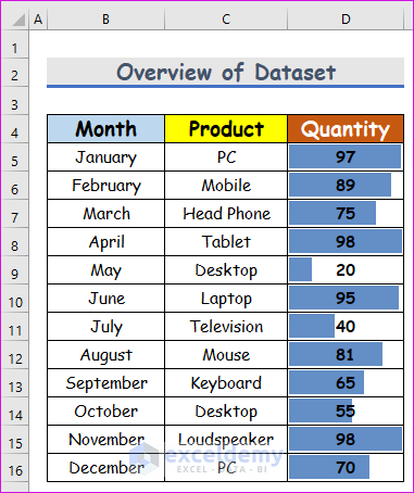
Let us have a data set like this. We consider a dataset of the product types, months, and quantities of those products given in columns C, B, and D, respectively. Using this dataset, we will create a blue data bar with the help of the Conditional Formatting option in Excel. Here’s an overview of the dataset for today’s task.

1. Use Solid Fill Command with Conditional Formatting to Add Blue Data Bar

In this section, we will use the Solid Fill command from the Conditional Formatting option to add a blue data bar in Excel. From our dataset, we will create a blue data bar to understand the quantity of the products. Let’s follow the instructions below to add a blue data bar!

Steps:

• First of all, select cells where we want to add a blue data bar. From our dataset, we select cells from D5 to D16. Then, from your Home tab, go to,

Home → Styles → Conditional Formatting → Data Bars → Solid Fill

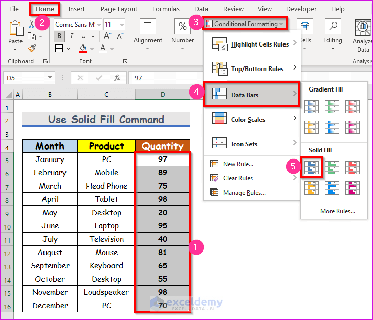
• Hence, from the Solid Fill option, we will select the blue color data bar.
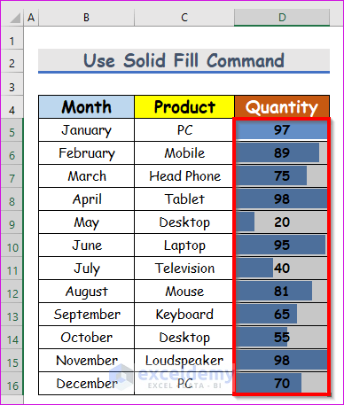
• Finally, we will be able to create a blue data bar which has been given in the below screenshot.

Read More: How to Add Solid Fill Data Bars in Excel (2 Simple Methods)

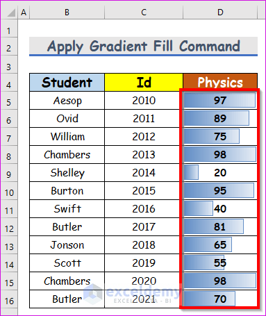
2. Apply Gradient Fill Command with Conditional Formatting to Add Blue Data Bar

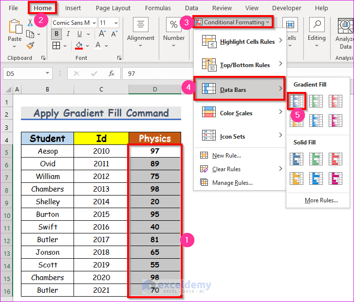
Conditional formatting is a good practice for highlighting or creating a data bar. With the help of conditional formatting, you can create a blue data bar. Here, we will use the Gradient Fill command to add a blue data bar in a column heading with Physics. The procedure is stated below.

Steps:

• We will apply conditional formatting. Firstly, from our dataset, select cells from D5 to D16 for the convenience of our work. After that, from your Home tab, go to,

Home → Styles → Conditional Formatting → Data Bars → Gradient Fill

• As a result, you will be able to create a Gradient Fill type blue data bar.

Read More: Conditional Formatting Data Bars Different Colors

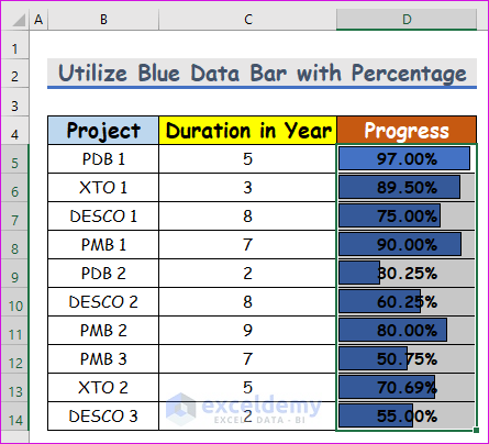
3. Utilize Blue Data Bar with Percentage in Excel

Last but not least, in this method, we consider a dataset of the working progress of 10 identical projects. The name of the projects is in column B, their duration is in column C, and the progress rate is in column D. So, our dataset is in the range of cells B5:D14.

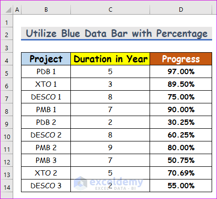
From our dataset, we will create a blue data bar with the percentage. Let’s follow the instructions below to learn!

Steps:

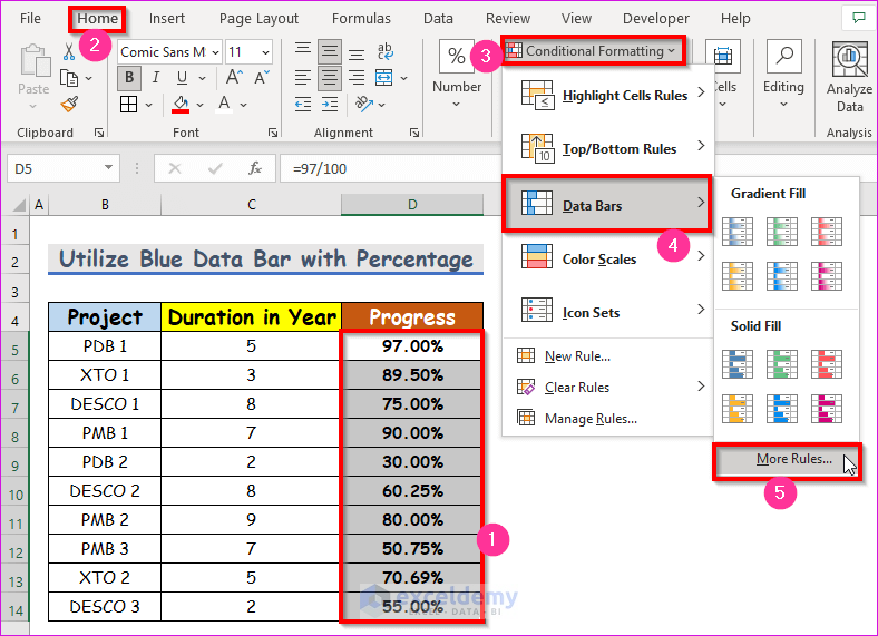
• Firstly, select cells from D5 to D14. After that, from your Home tab, go to,

Home → Styles → Conditional Formatting → Data Bars → More Rules

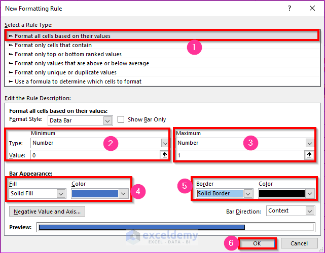
• A dialog box named New Formatting Rule will appear. Follow the steps for the New Formatting Rule dialog box. Firstly, select Format all cells based on their values.
• After that, change the Type of Minimum option from Automatic to Number, and denote the Value of the Minimum field as 0.
• Similarly, set the Type and the Value option for the Maximum field.
• Hence, in the Bar Appearance section, choose the bar style according to your desire. We choose the Solid Fill option in the Fill field and the Blue, Accent 1 color in the Color field.
• Further, select the Solid Border option in the Border field and the Black color in the Color field.
• At last, press the OK option.

• After completing the above process, you will be able to create a blue data bar.

Read More: [Fixed]: Conditional Formatting in Data Bar Percentage Not Working in Excel

Conclusion

I hope all of the suitable methods mentioned above to add a blue data bar will now encourage you to apply them in your Excel spreadsheets with more productivity. You are most welcome to feel free to comment if you have any questions or queries.