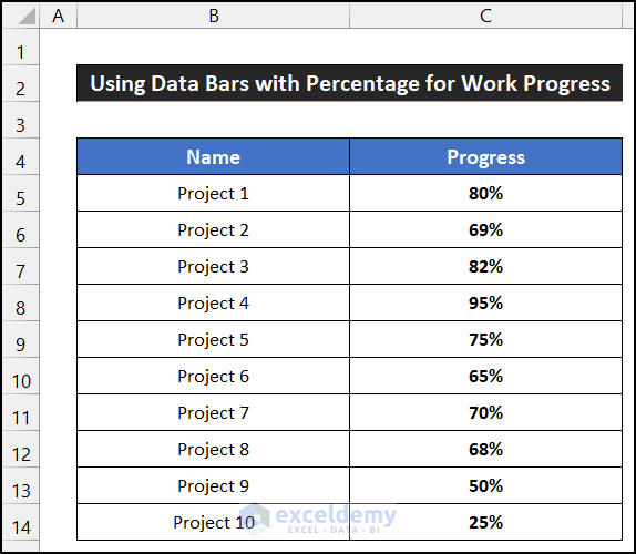
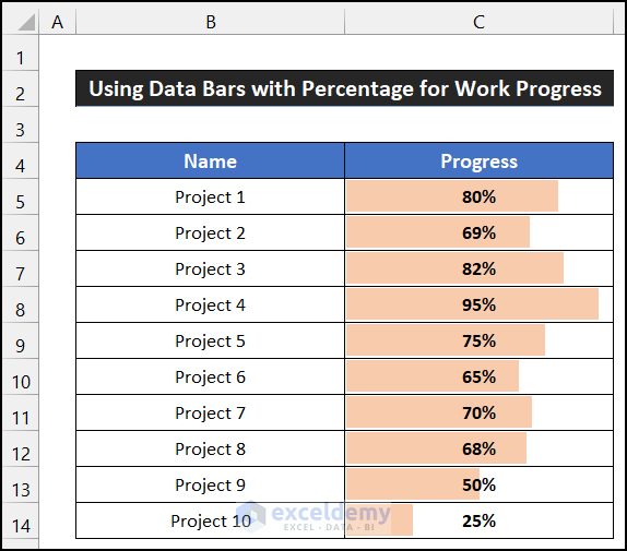
Example 1 – Using Data Bars with Percentage for Work Progress
Consider a dataset representing the working progress of ten identical projects. The project names are in column B, and their progress rates are in column C (cells B5:C14).
Follow these steps:
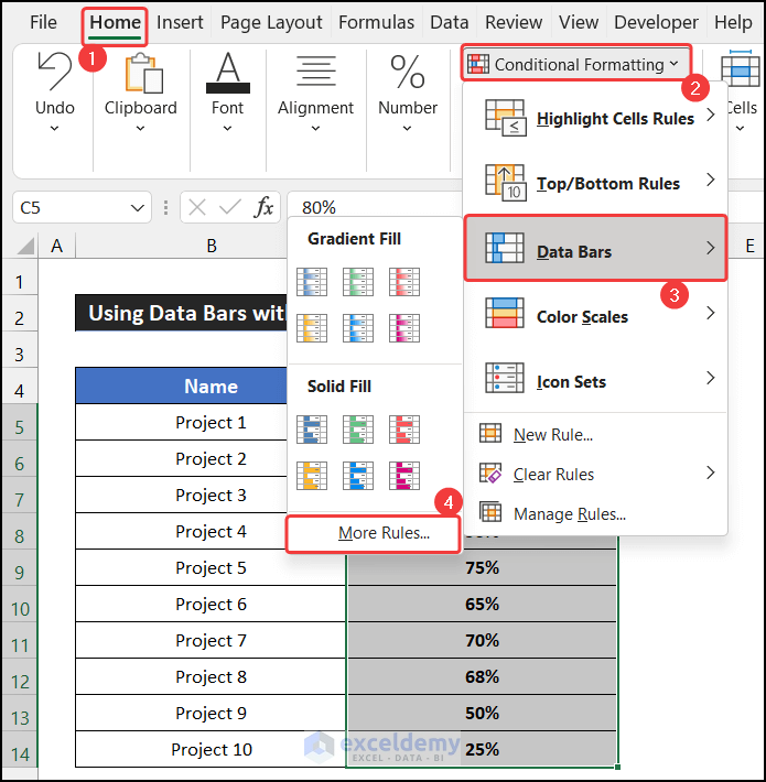
- Select the range of cells C5:C14.
- In the Home tab, click on the drop-down arrow of the Conditional Formatting option from the Styles group.
- Choose the More Rules option from the Data Bars section.
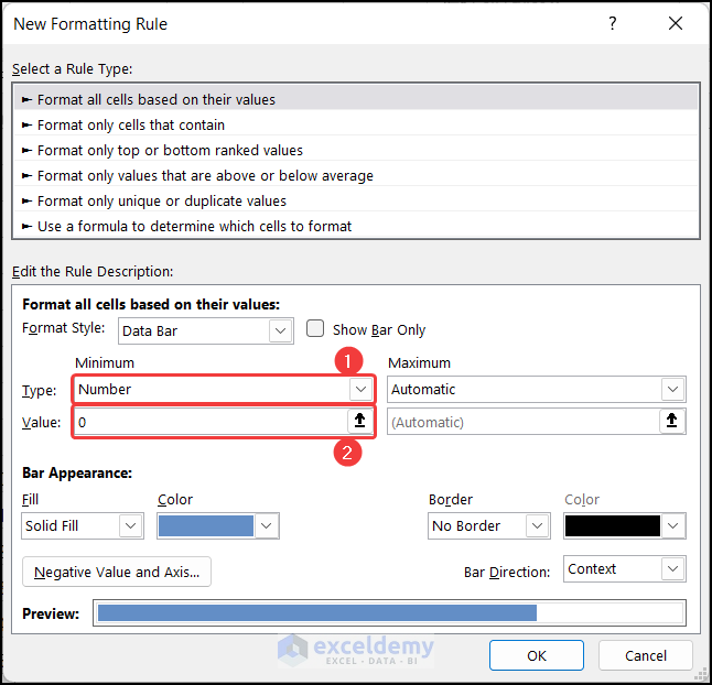
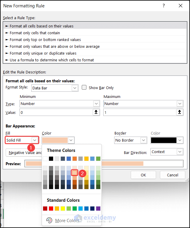
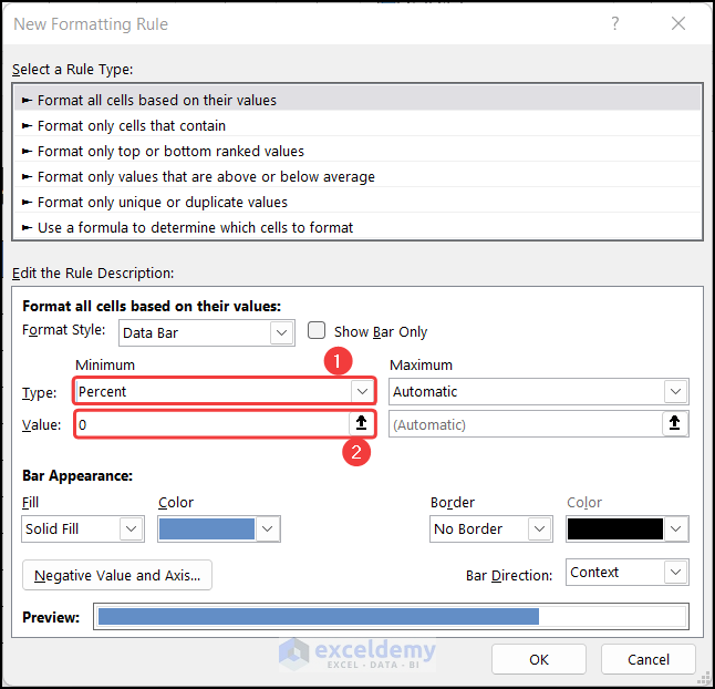
- In the resulting dialog box (New Formatting Rule), change the Type of Minimum from Automatic to Number.
- Set the Value of the Minimum field to 0.
- Similarly, configure the Type and the Value option for the Maximum field.
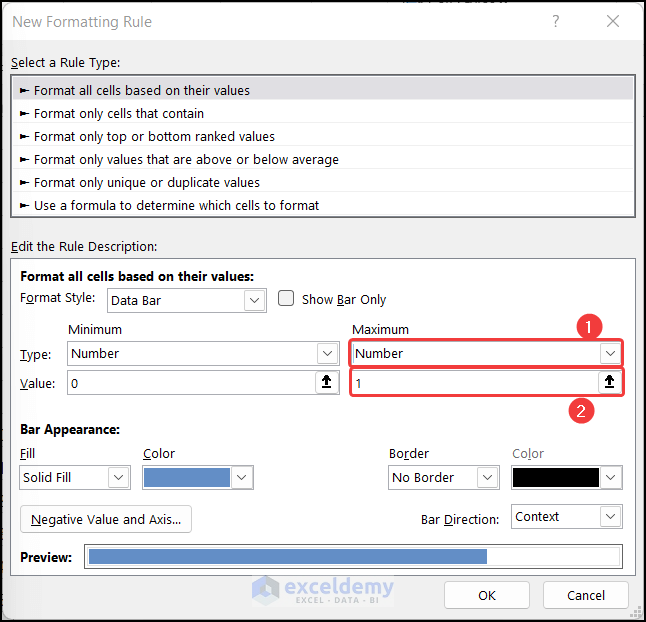
- Customize the bar appearance (e.g., Solid Fill with an Orange, Accent 2, Lighter 60% color).
- Click OK to apply the data bar formatting based on the values.
- You will notice the cells will get the data bar formatting according to the values.
Read More: Conditional Formatting Data Bars Different Colors
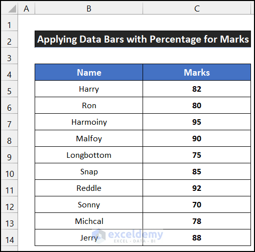
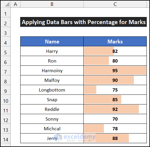
Example 2 – Applying Data Bars with Percentage for Marks
Consider a dataset of examination marks for ten students. Student names are in column B, and their marks are in column C (cells B5:C14).
Follow these steps:
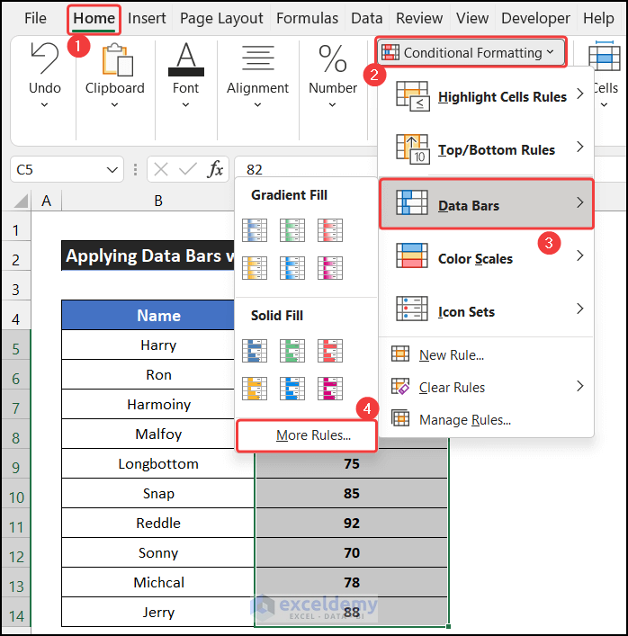
- Select the range of cells C5:C14.
- In the Home tab, click on the drop-down arrow of the Conditional Formatting option from the Styles group.
- Choose the More Rules option from the Data Bars section.
- In the dialog box, change the Type of Minimum from Automatic to Percent.
- Set the Value of the Minimum field as 0.
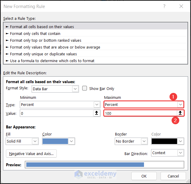
- Configure the Type as Percent and set the Value option as 100 for the Maximum field.
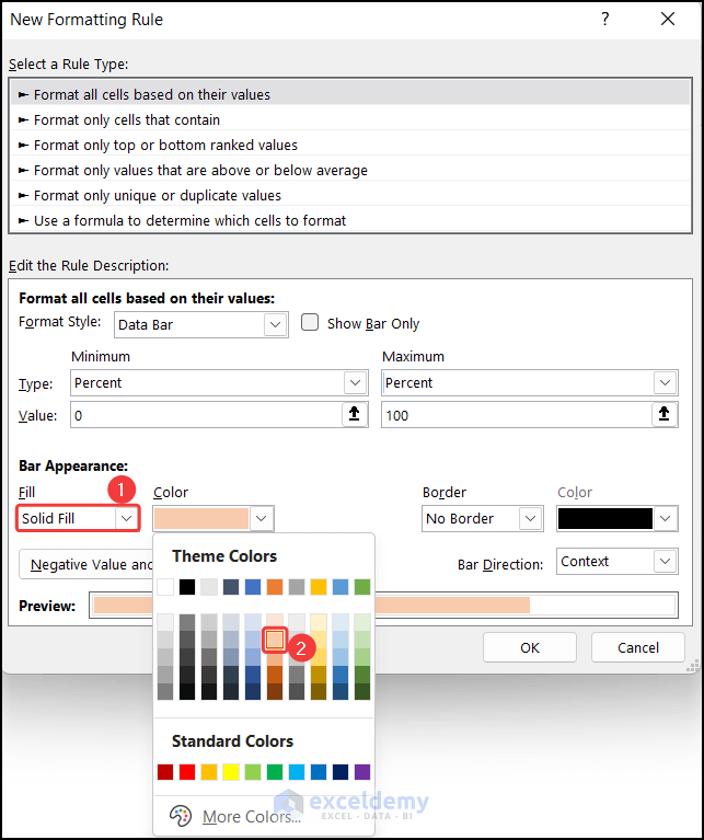
- Customize the Bar Appearance (e.g., Solid Fill with an Orange, Accent 2, Lighter 60% color).
- Click OK to apply data bars with percentage formatting.
- You will notice that all the cells will get the data bars percentage formatting according to the values.
Read More: Conditional Formatting with Data Bars Based on Another Cell in Excel
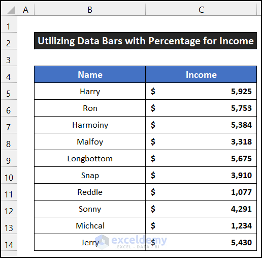
Example 3 – Utilizing Data Bars with Percentage for Income
In this example, we’ll focus on income data for ten employees during a specific month. The employees’ names are in column B, and their income figures are in column C (cells B5:C14).
Follow these steps:
- Select the range of cells C5:C14.
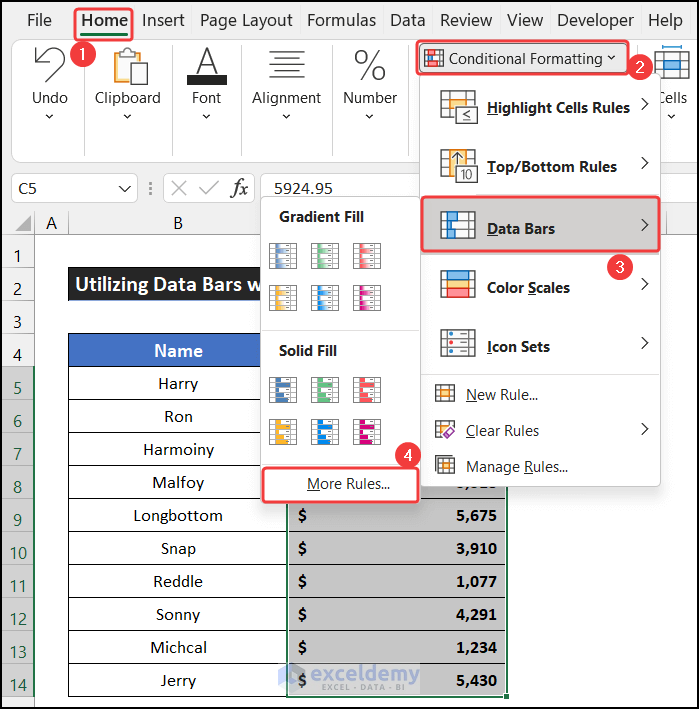
- In the Home tab, click on the drop-down arrow of the Conditional Formatting option from the Styles group.
- Choose the More Rules option from the Data Bars section.
- In the resulting dialog box (New Formatting Rule), change the Type of Minimum from Automatic to Percent.
- Set the Value of the Minimum field as 0.
- Configure the Type as Percent and set the Value option to 100 for the Maximum field.
- Customize the bar appearance (e.g., Solid Fill with an Orange, Accent 2, Lighter 60% color).
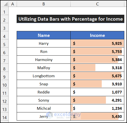
- Click OK to apply data bars with percentage formatting.
- You will see that all the cells will get the data bar percentage formatting according to the values.
Read More: How to Add Data Bars in Excel
Download Practice Workbook
You can download the practice workbook from here:
Related Articles
- [Fixed]: Conditional Formatting in Data Bar Percentage Not Working in Excel
- How to Define Maximum Data Bars Value in Excel
- How to Add Solid Fill Data Bars in Excel
<< Go Back to Data Bars | Conditional Formatting | Learn Excel
Get FREE Advanced Excel Exercises with Solutions!
