Looking for ways to define maximum Data Bars value in Excel? Then this is the right article for you. Data Bar is a Conditional Formatting feature inside Excel that gets larger for more extensive data. We use this to compare data against other data in Excel. In this article, we will show you 6 easy methods to define maximum Data Bars value in Excel.
How to Define Maximum Data Bars Value in Excel: 6 Handy Approaches
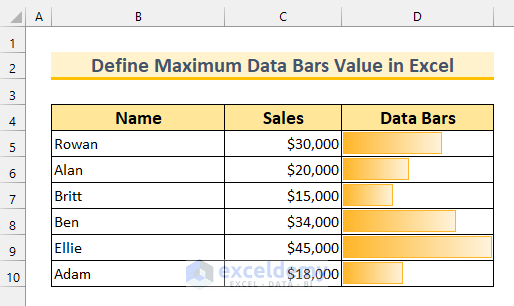
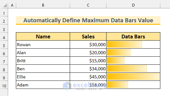
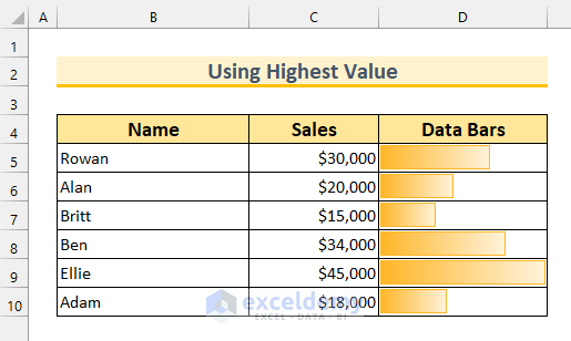
To demonstrate our methods, we have selected a dataset with 3 columns: “Name”, “Sales”, and “Data Bars”. We have used the sales data to create a “Data Bar” and we will set the maximum value using 6 options.
1. Define Maximum Data Bars Value in Excel Automatically
For the first method, we will use the Automatic feature to define the maximum Data Bar value in Excel.
- To begin with, copy all the sales values into the next column.
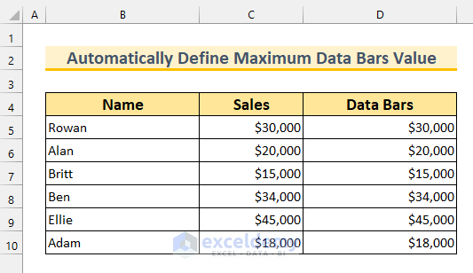
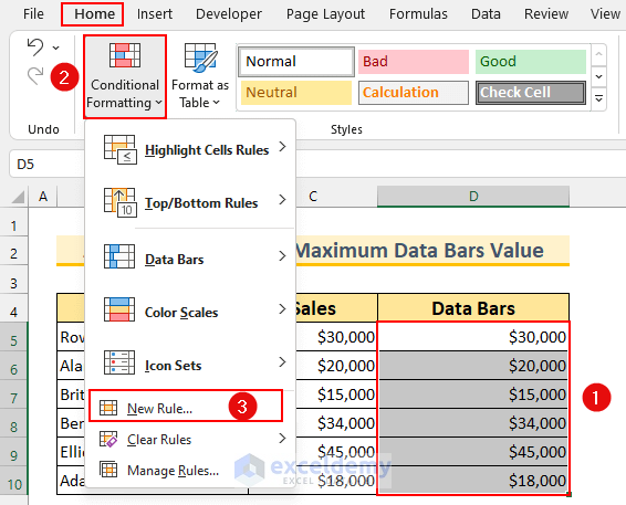
- Then, select the cell range D5:D10.
- Next, from the Home tab >>> Conditional Formatting >>> select “New Rule…”.
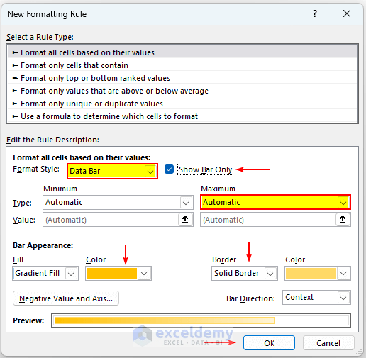
- So, the New Formatting Rule dialog box will pop up.
- Then, select Data Bar from the Format style box.
- Afterward, select Show Bar Only. This will hide the numbers from the Data Bars.
- Then, under the Maximum, select Automatic as the Type.
- Optionally, you can change the Bar Appearance using Fill and Border color.
- After that, press OK.
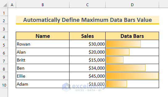
- So, our Data Bars will look like this.
- Additionally, we can add preset to the Data Bars.
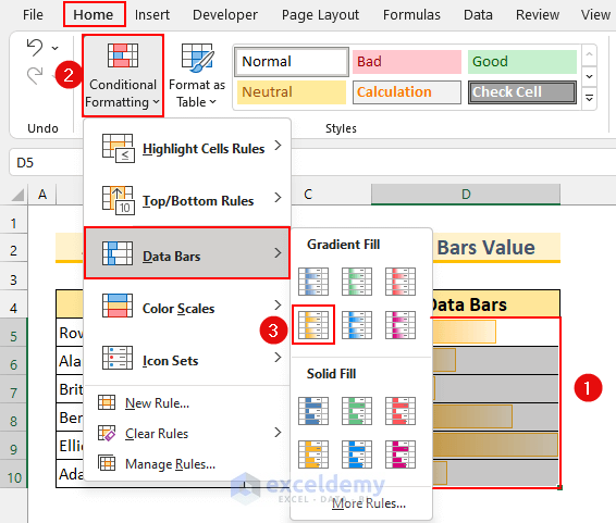
- To do so, select the Data Bars.
- Then, from the Home tab >>> Conditional Formatting >>> Data Bars >>> select the Orange Data Bar preset.
- Lastly, our Data Bars will look like this and we have defined the maximum value as Automatic.
Read More: Conditional Formatting Data Bars Different Colors
2. Using Highest Value to Define Maximum Data Bars Value in Excel
For the second method, we will use the Highest Value option to define the maximum Data Bars value.
- Firstly, as shown in the first method, we have shown the Data Bars.
- Next, select the cell range D5:D10.
- Then, from the Data tab >>> Conditional Formatting >>> select Manage Rules.

- After that, the “Conditional Formatting Rules Manager” box will appear.
- Then, double-click on the Data Bar Rule.

- So, another dialog box will pop up.
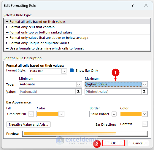
- Then, select the Highest Value from the Maximum Type.
- Lastly, press OK.
- Thus, we will change the maximum Data Bars value in Excel and the final step will return this result.
Read More: Conditional Formatting with Data Bars Based on Another Cell in Excel
3. Applying Number to Define Maximum Data Bars Value
For the third method, we will set a Number manually to define the maximum Data Bars value.
Steps:
- Firstly, as shown in the first method, we have shown the Data Bars.
- Then, similar to the second method, we bring up the Edit Formatting Rules dialog box.
- Next, select Maximum Type: Number.
- After that, set Maximum Value: 50,000.
- Lastly, press OK.

- So, the final output will be this.

Read More: How to Add Data Bars in Excel
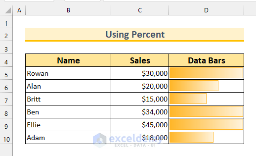
4. Define Maximum Data Bars Value in Excel Using Percent
For the fourth method, we will use Percent to set the maximum Data Bars value.
Steps:
- Firstly, as shown in the first method, we have shown the Data Bars.
- Then, similar to the second method, we bring up the Edit Formatting Rules dialog box.
- Next, select Maximum Type: Percent.
- After that, set the Maximum Value: 50.
- Lastly, press OK.

- So, the final output will be this as shown in the image below.
Read More: How to Use Data Bars with Percentage in Excel
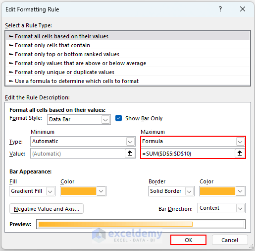
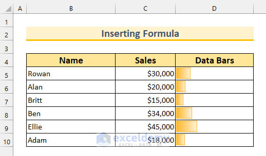
5. Define Maximum Data Bars Value Applying Formula
For the fifth method, we will use the SUM function to create a Formula to set the maximum Data Bar value in Excel.
Steps:
- Firstly, as shown in the first method, we have shown the Data Bars.
- Then, similar to the second method, we bring up the Edit Formatting Rules dialog box.
- Next, select Maximum Type: Formula.
- After that, set Maximum Value: type this formula from below.
=SUM($D$5:$D$10)
- This formula sets the Data Bars as the proportion of the total sales amount.
- Lastly, press OK.
- Hence, the final output will be this.
6. Using Percentile to Define Maximum Data Bars Value
For the last method, we will use the Percentile feature to set the maximum Data Bars value.
Steps:
- Firstly, as shown in the first method, we have shown the Data Bars.
- Then, similar to the second method, we bring up the Edit Formatting Rules dialog box.
- Next, select Maximum Type: Percentile.
- After that, set the Maximum Value: 90.
- Lastly, press OK.

- Consequently, the modified Data Bars will be like this.

Read More: [Fixed]: Conditional Formatting in Data Bar Percentage Not Working in Excel
Practice Section
We have added a practice dataset for each method in the Excel file. Therefore, you can follow along with our methods easily.

Download Practice Workbook
Conclusion
We have shown you 6 handy approaches to how to define maximum Data Bars value in Excel. If you face any problems regarding these methods or have any feedback for me, feel free to comment below. Thanks for reading, keep excelling!
Related Articles
- How to Add Solid Fill Data Bars in Excel
- How to Add Blue Data Bar in Excel
- How to Remove Data Bars in Excel
- [Solved]: Data Bars Not Working in Excel
<< Go Back to Data Bars | Conditional Formatting | Learn Excel
Get FREE Advanced Excel Exercises with Solutions!
