How to Remove Data Bars in Excel (3 Simple Ways)

While working in Microsoft Excel we need to highlight cells or highlight data inside a chart. Sometimes, we use data bar rules of conditional formatting to highlight cells. We also insert charts to visualize the values of the cells. However, it becomes difficult to remove data bars from both cells and charts. In this article, I am describing how to remove data bars in Excel.

How to Remove Data Bars in Excel: 3 Easy Ways

In the following article, I am describing 3 simple and easy ways to remove data bars in Excel.

Suppose, we have a dataset of some Student Names and their Total Scored Marks in different subjects. Now, we are going to visualize them with data bars and remove some data bars using Excel’s built-in feature.

1. Use Conditional Formatting to Remove Data Bars in Excel

Often you will find data tables with applied data bar rules using conditional formatting. It is very easy to remove those data bars from the cells. To do so-

Steps:

First, select cells (D5:D12) as these cells have data bars.
While the cells are selected click “Conditional Formatting” from the home ribbon.

Then, press “Clear Rules from Selected Cells” from the “Clear Rules” option.

In conclusion, all the data bars will be removed from the cells.

2. Delete Rows to Remove Data Bars in Excel

In the previous method, I removed bars using conditional formatting. But this won’t work for an inserted chart. But I have a solution for the charts. Follow the steps below-

Step 1:

In general, choose cells that you want to visualize inside the chart. Here I have selected cells (C4:D12).
While the cells are selected choose the “Chart” from the “Insert” option.

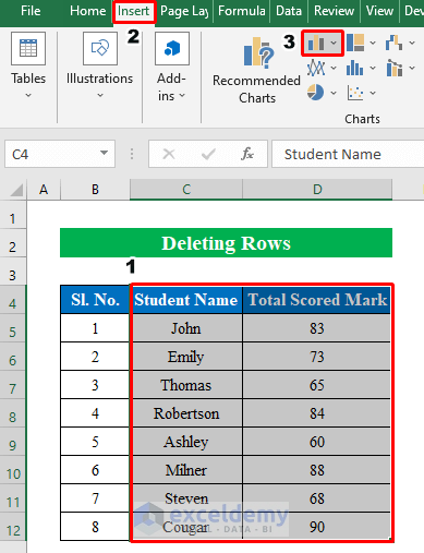
Therefore, from the drop-down list click a “2-D Bar Chart”.

Eventually, a data bar will be created. Now, let’s remove some data bars from the chart.

Step 2:

To delete bars from the chart first select some rows from the table by holding the Ctrl button.

In the meantime, click the right button on the mouse and press “Delete” from the options.

Thus, the data bars will be removed from both the chart and the table.

3. Utilize Select Data Option to Remove Data Bars in Excel

Sometimes you might need to remove the data bars only from the chart at the same time the values will be available on the dataset. Follow the steps below-

Step 1:

Above all, let’s start with creating the chart.
Choose cells (C4:D12) and click “Recommended Charts” from the “Insert” option.

Hence, a new window will pop up named “Insert Chart”.
First of all, click “All Charts” and choose a “Clustered Column” chart from the “Column” option.
Press OK to continue.

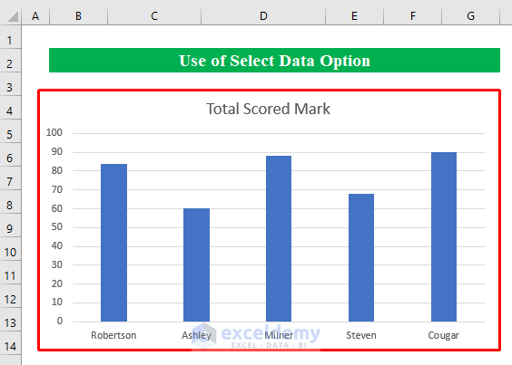
Hereafter, our chart is prepared by visualizing all the values from the table.

Step 2:

Upon selecting the chart press the right button of the mouse and choose “Select Data”.

Next, uncheck some “Names” from the “Horizontal Axis Labels”.
Hit the OK button to continue.

Finally, we have successfully removed the data bars of our choice from the chart.

Things to Remember

Data bars look good if there is less variation in the data and it only plots for quantitative values.

Download Practice Workbook

Download this practice workbook to exercise while you are reading this article.

Remove Data Bars.xlsx

Conclusion

In this article, I have tried to cover all the effective methods to remove data bars in Excel. Take a tour of the practice workbook and download the file to practice by yourself. I hope you find it helpful. Please inform us in the comment section about your experience.