Data bars are the graphical representation of values of a dataset in Excel. They add an upgraded dimension to your worksheet in terms of presentation, clarification of information, and lots more. In this article, you will learn how to add data bars in Excel with 2 easy methods. Let’s go ahead.
How to Add Data Bars in Excel: 2 Easy Methods
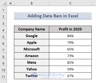
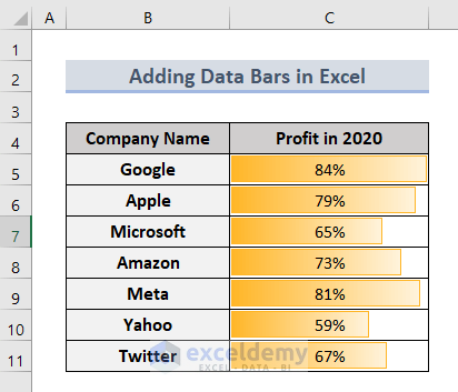
To illustrate the 2 methods to add data bars, we have prepared a dataset. It shows the profits of 7 companies in the year 2020. We will illustrate this data through data bars here which will benefit us to get a graphical comparison.
Let’s look at the following methods to add data bars:
Method 1: Add Data Bars with Conditional Formatting in Excel
Conditional Formatting is a useful tool that helps Excel users change the appearance of a dataset based on certain conditions or criteria such as minimum or maximum numbers, range of values, etc. Here, we will see the first method to add data bars with Conditional Formatting in Excel. To conduct this, follow the steps below:
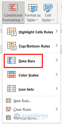
- Secondly, on the Home tab, go to the Styles section>> click on Conditional Formatting.

- Then, select Data Bars from the Conditional Formatting drop-down section.
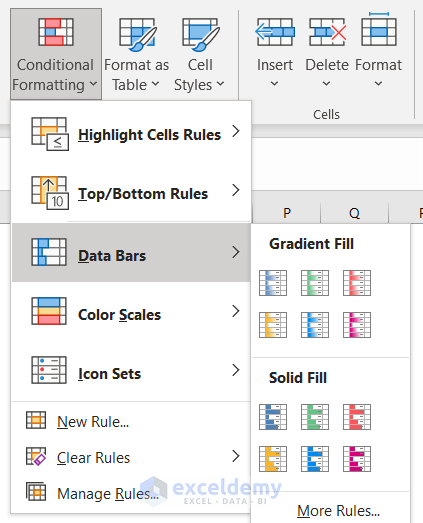
- After that, select any type of bar style from the options here.
- That’s it, you have successfully added data bars to your dataset. It is shown inside the range that you selected in the beginning.
- Now, we will check if the data bar is working or not.
- For example, we changed the value in cell C8. You can see that the bar length changed automatically according to its value.

Note: Data Bars are also applicable for negative values. It will just show the bar red in the opposite direction like this:

Method 2: Use Excel VBA Macro to Add Data Bars
Another process to add data bars in Excel is to use VBA Macro. In this method, we will be doing conditional formatting just like before but in the Format Conditions in the Macro. Let’s follow the steps below to add data bars in the same dataset:
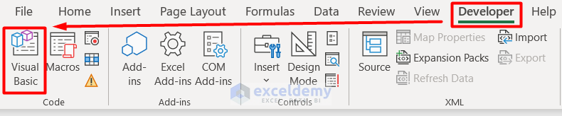
- Initially, press Alt+F11 or select the Visual Basic feature from the Developer tab.
- Then, go to Insert and select Module.
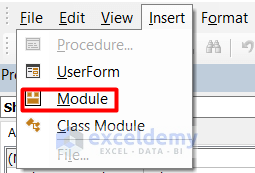
- After that, a new blank page will appear.
- Insert this VBA code inside this page.
Sub databarsfc()
Dim dtrg As Range
Dim dtdb As databar
Set dtrg = Range("C5", Range("C11").End(xlDown))
Set dtdb = dtrg.FormatConditions.AddDatabar
With db
    'pos bar formatted with blue gradient & blue border
    .BarColor.Color = vbBlue
    .BarFillType = xlDataBarFillGradient
    .BarBorder.Type = xlDataBarBorderSolid
    .BarBorder.Color.Color = vbBlue
    'the axis set automatically and coloured red
    .AxisPosition = xlDataBarAxisAutomatic
    .AxisColor.Color = vbRed
    'the neg bar formatted with red gradient and red border
    With .NegativeBarFormat
        .ColorType = xlDataBarColor
        .Color.Color = vbRed
        .BorderColorType = xlDataBarColor
        .BorderColor.Color = vbRed
    End With
End With
End Sub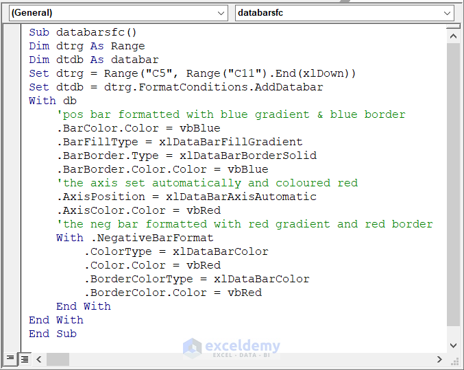
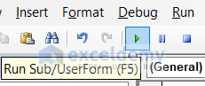
- Now, press the F5 key on your keyboard or select the RunSub button from the upper layer.
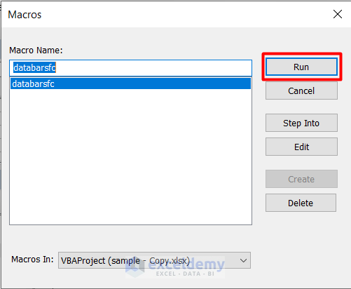
- You will be directed to the Macros window.
- Here, click on Run.
- Finally, we have completed the task of adding data bars in Excel.

- You can customize these data bars by adding more commands for conditional formatting in the VBA macro. The opportunity expands to changing colors, value, appearance, etc.
Note: Here is another option for the VBA code for you.
Sub DataBarFormatting()
Dim DataRange As Range
Set DataRange = Range(“C5, C11”)
DataRange.FormatConditions.Delete
DataRange.FormatConditions.AddDatabar
End Sub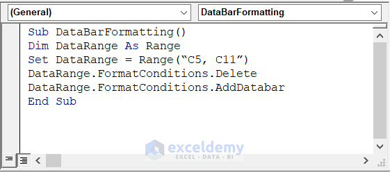
Read More: How to Add Blue Data Bar in Excel
How to Customize Added Data Bars in Excel
In this section, we will see a quick guide on how to customize added data bars on conditional formatting in Excel. Let’s follow the steps:
- First, complete Method 1 as described above.
- After that, select the whole range of datasets with data bars.

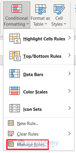
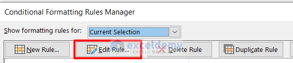
- Then, go to Conditional Formatting from the Home tab and select Manage Rules.
- Here, click on Edit Rule.
- Finally, you can see that a new Edit Formatting Rule window appeared.
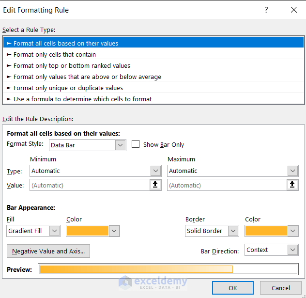
- In this window, customize your data bar according to your preference in terms of color, value, appearance, etc.
Read More: Conditional Formatting Data Bars Different Colors
How to Clear Data Bars in Excel
After adding data bars, you may need to get back to the previous look. For this just go through the process below:
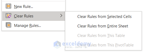
- Select Clear Rules from the drop-down section of Conditional Formatting.

- Now, choose any of the options to clear data bars depending on your preference.
Read More: How to Remove Data Bars in Excel
Things to Remember
- Data Bars are applicable for values, not any data in text format.
- It is different from Charts because Data Bars work only through the horizontal axis.
- It would be better if you worked with around 100 datasets because it may cause difficulty in interpreting the data bar in Excel.
- In the case of working with VBA code, keep in mind that, it will always keep the lowest value cell blank. It means there will be no data bar for the least value.
Download Workbook
Get the sample workbook here and practice.
Conclusion
So, in this article, we have seen 2 methods to add data bars in Excel. We also explored the possibilities of customization. Hope this was a helpful one. Waiting for your generous suggestions.
Related Articles
- How to Use Data Bars with Percentage in Excel
- How to Define Maximum Data Bars Value in Excel
- [Solved]: Data Bars Not Working in Excel
- Conditional Formatting with Data Bars Based on Another Cell in Excel
- [Fixed]: Conditional Formatting in Data Bar Percentage Not Working in Excel
- How to Add Solid Fill Data Bars in Excel
<< Go Back to Data Bars | Conditional Formatting | Learn Excel
Get FREE Advanced Excel Exercises with Solutions!
