How to Use Conditional Formatting Icon Sets?

This article will summarize all the possible cases in conditional formatting icon sets in Excel. In this Excel tutorial, you will learn about
– Different types of conditional formatting icon sets on other cells’ values
– Using conditional formatting icon sets using formulas
– Displaying two columns’ comparisons using these icon sets
– How to use them for texts

We have used Microsoft 365 for the examples and applications. However, they are also applicable to other versions too.

“Icon sets” are used as a performance indicator, progress tracking, risk assessment, comparison and analysis, and so on. They are also helpful for visualizing a cluster of data.

Download Practice Workbook

How to Use Conditional Formatting Icon Sets in Excel?

We can use icon sets to define a range of cells based on certain criteria. To use icon sets, we can use the Icon Sets option from Conditional Formatting.

• Select the defined cells and go to the Home tab.
• From the ribbon, go to Conditional Formatting and click on Icon Sets.
• After that, pick an icon set according to your preference.

What Are Some Uses of Conditional Formatting Icon Sets in Excel? (4 Applications)

We can apply conditional formatting icon sets in different cases based on our necessity. Here are 4 of the most used cases described in detail.

1. Conditional Formatting Icon Sets Based on Another Cell Value

We can use the IF function with the Conditional Formatting feature to set conditional formatting icon sets based on another cell.

1.1. Insert Shapes Conditional Formatting Icon Sets Based on Another Cell

• We can use different shapes of icons as conditional formatting icon sets based on another cell. To do so, remark the values in the Marks column with conditional values using the following formula.

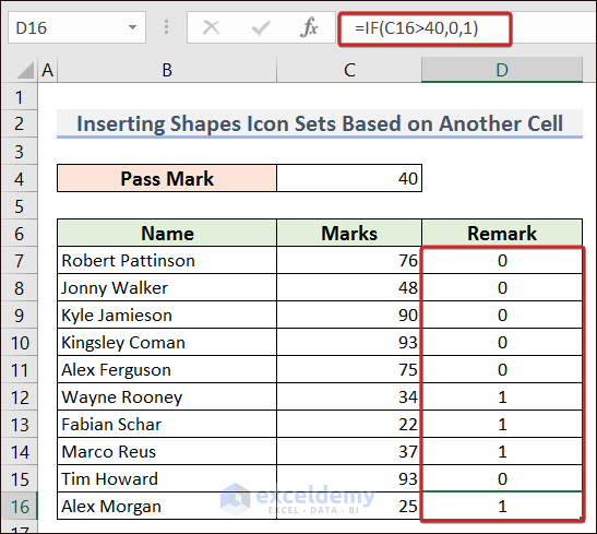
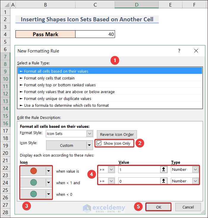
• Then from the New Formatting Rule wizard, select Format all cells based on their values from Select a Rule Type. You can check the Show icon only box to have just an icon and remove the remark numbers.
• Select icon shapes and insert conditions. Click OK to finish the process.

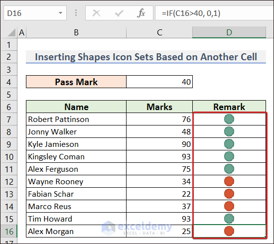
• You will have just shapes as conditional formatting icon sets.

1.2. Insert Indicators Icon Sets Based on Another Cell

• You can remark the percentage values in the completion column with conditional values using the IFS function in the following formula.

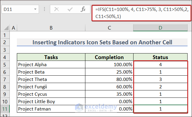
• Open the New Formatting Rule wizard and select Format all cells based on their values from Select a Rule Type.
• Pick an indicator pattern for conditional formatting icon sets. You can check the Show icon only box to have just the indicator icons and remove the remark numbers.
• Insert the conditions and click OK.

• Thus, indicators will be set as conditional formatting icon sets based on another cell.

1.3. Insert Directional Icon Sets Based on Another Cell

• We can insert different directional icons as conditional formatting icon sets based on another cell. For this, remark the values in the Change in Market Value column with conditional values using the following formula.

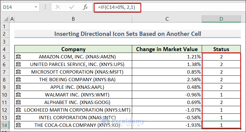
• Then from the New Formatting Rule wizard, select Format all cells based on their values from Select a Rule Type.
• You can check the Show icon only box to have just the icons and remove the remark numbers.
• Pick the directional icons and insert conditions. Click OK to finish the process.

• Thus, We can insert directional conditional formatting icon sets based on another cell

1.4. Insert Rating Icon Sets Based on Another Cell

• You can remark the sales values of the Total Sales column with conditional values in the Ratings column using the following formula.

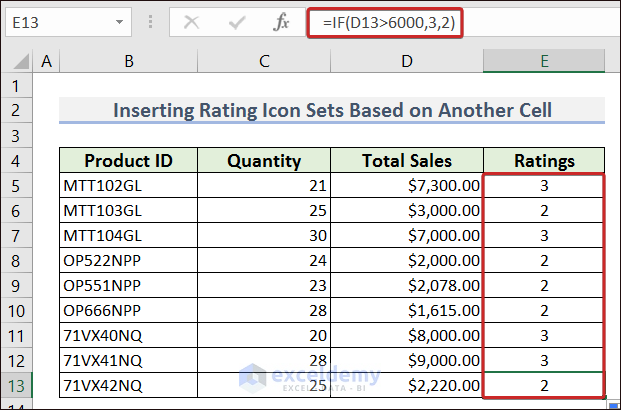
• Pick your rating icon sets and insert conditions. Click OK to finish the entire process.

• You will have the rating icons as conditional formatting icon sets based on another cell.

2. Apply Formula for Conditional Formatting Icon Sets

We can apply a complete formula with the AVERAGE function as the condition for conditional formatting icon sets.
For this, I have a dataset with examination marks where I want to set icons based on the average mark value.

• As I want to mark green the cells having a value equal to or more than 20 of the average value, I have applied the following formula in the Value section.

• Again, I want to mark yellow the cells having equal or less than 10 of the average mark. Just apply the following formula.

• I have set the rest of the cells as red. Click OK to finish the procedure.

• Finally, we have our defined icons on the Marks column based on the formula.

3. Conditional Formatting Icon Sets to Compare Two Columns

In order to use conditional formatting icon sets to compare two columns, find the difference between those columns in percentage and use those values in conditional formatting.

• Apply the following formula in column E to find the difference in the values of those two columns.

• Then, set the directional icon sets as conditional formatting icon sets. For a difference greater than 0%, it will set the green icon. The yellow icon will be set for 0% difference and the rest cells will have the red icon.

• Finally, you have the comparison of columns C and D with conditional formatting icon sets.

4. Conditional Formatting Icon Sets Based on Text

You can use the combination of the IFS and VLOOKUP functions or the COUNTBLANK function to have a remark as a text of a certain value. You can use that remark in conditional formatting to define the icon sets.

4.1. Conditional Formatting 3 Icon Sets Based on Text

• In order to add 3 icon sets of conditional formatting based on text, I have applied the following formula to define the examination marks of column C in the text format in column D.

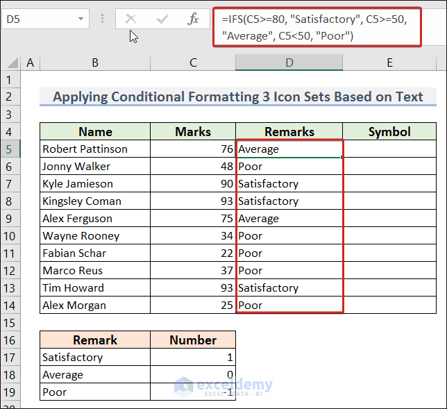
• After that, I applied a formula with the VLOOKUP function to remark the text of column D into the number in column E.

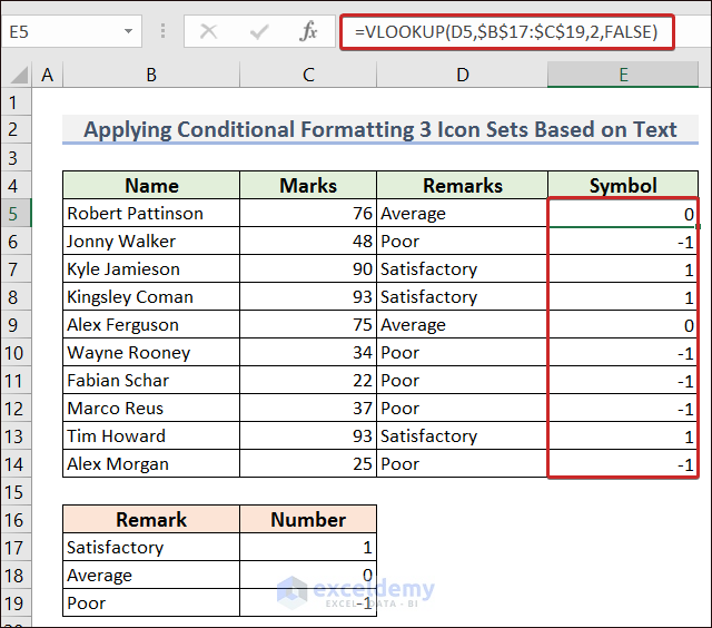
• Then set icons and conditions from the Conditional Formatting option. Click OK and finish the process.

• Thus, we can have conditional formatting of 3 icon sets based on text.

4.2. Conditional Formatting 5 Icon Sets Based on Text

• For conditional formatting, 5 icon sets based on text, apply the following formula first in column D to define the marks in the text.

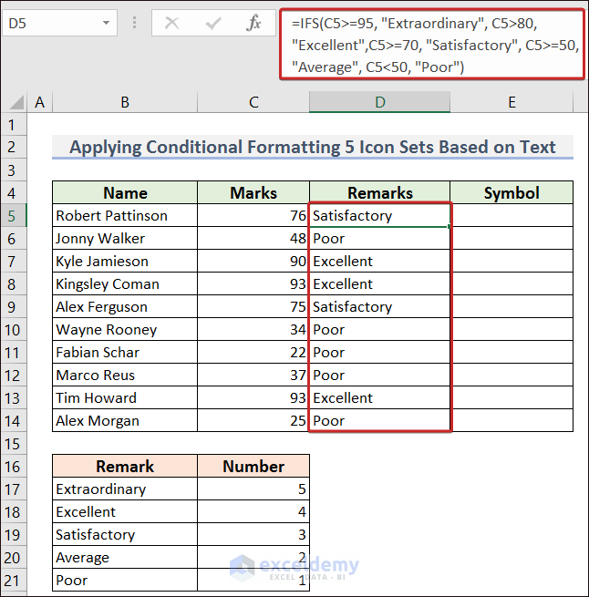
• Next, define the text of column D into a number in column E with the following formula.

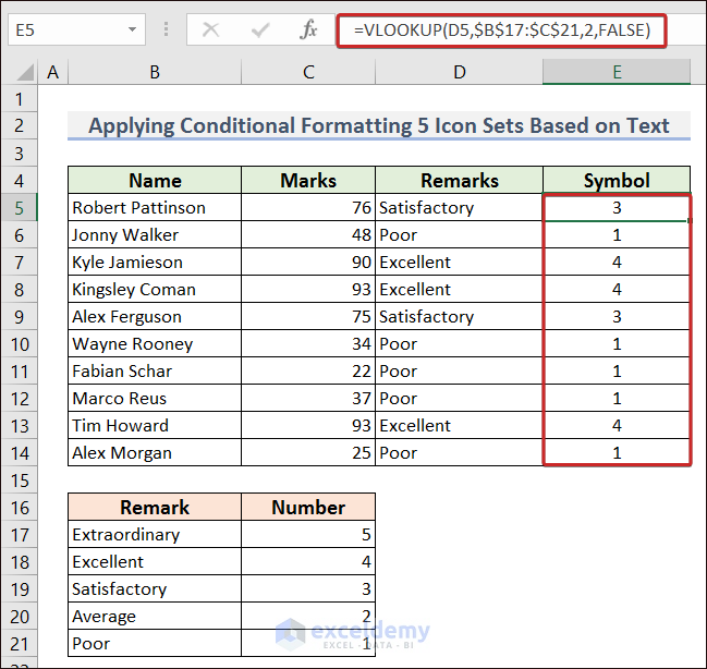
• Now select a 5-set icon and set the condition for each icon. Apply the conditional formatting just by clicking the OK button.

• We will have the conditional formatting of 5 icon sets based on text.

4.3. Icon Sets Based on Blank or Non-Blank Cells

• To count the blank cells, apply the following formula with the COUNTBLANK function in column E.

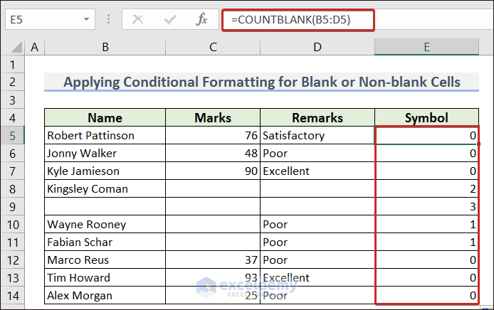
• Then set icons and conditions from the Conditional Formatting option. Click OK and finish the process.

• Thus, we can have conditional formatting icon sets based on the number of blank or non-blank cells.

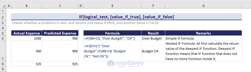
How to Create Custom Conditional Formatting Icon Sets in Excel?

The IF function is a useful tool for creating conditional formatting icon sets in Excel. It checks whether a condition is met, and returns one value if TRUE, and another value is FALSE.

• In order to create custom icon sets in Excel, go to the Insert tab.
• Then select Symbol from the Symbols option in the ribbon.

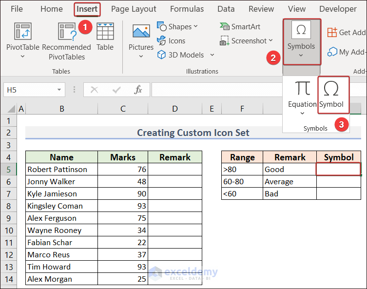
• Pick an icon according to your choice and press Insert to have it in the selected cell.

• Following similar procedures, insert as many icons as you need.

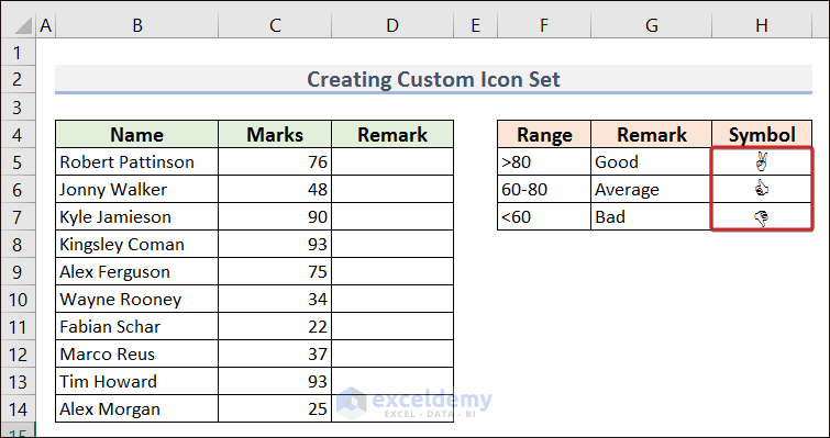
• Now, apply the following formula in column D. You will have some characters based on the matched conditions.

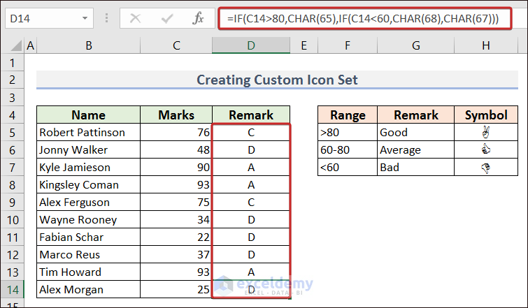
• Now select cells in column D and change the font matching the symbol (i.e. Windings) and thus, we will have custom conditional formatting icon sets in Excel.

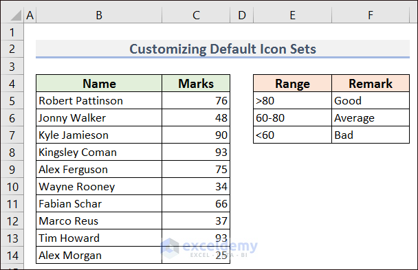
How to Customize Default Conditional Formatting Icon Sets in Excel?

We can customize the default conditional formatting icon sets with the Icon Style option from the New Formatting Rule wizard.

• In order to go deep on how to customize default conditional formatting icon sets, consider a dataset and conditions first.

• Then go according to the following instructions to apply them.

Select Cells —> Home Tab —> Conditional Formatting —> Icon Sets —> More Rules…

• A wizard named New Formatting Rule will appear.
• Pick an icon for every matched condition according to your choice and click OK to finish the process.

• We will have the customized icon sets instead of the default ones in cells C5:C14.

Frequently Asked Questions

1. Can we edit the applied conditional formatting icon sets?

Yes, we can certainly edit the applied conditional formatting icon sets. For this, select the cells having conditional formatting icon sets and go to the Manage Rules… option from Conditional Formatting. From there, you can easily edit the formula from the Edit option.

2. What are the types of conditional formatting?

There are 5 types of conditional formatting. They are- background color shading of cells, foreground color shading of fonts, icons, data bars, and values.

3. What is the default rule type for icon sets?

The three icons set is the default one in Excel. It separates the top, middle, and bottom thirds of a data range.

Conclusion

In the above sections, I have tried to summarize all the possible cases in Conditional Formatting Icon Sets in Excel. With this article, you will be able to learn the entire procedure to add conditional formatting icon sets. You will also learn the applications of conditional formatting icon sets based on different situations.

Based on your need, you can pick any of the described procedures to add conditional formatting icon sets. I hope this article will be helpful for you. For any further questions, please comment below. You can also visit our site for more Excel-related articles.

Conditional Formatting Icon Sets: Knowledge Hub

• Conditional Formatting Icon Sets Based on Text
• Conditional Formatting Icon Sets Based on Percentage
• Change Conditional Formatting Icon Set Color
• Conditional Formatting Icon Sets with Relative Reference
• Conditional Formatting with More than 3 Icon Sets
• Conditional Formatting: Add Custom Icon Sets
•  Conditional Formatting Icon Sets Based on Another Cell

<< Go Back to Conditional Formatting | Learn Excel