Excel Conditional Formatting Icon Sets with Relative Reference

While working with Microsoft Excel, to emphasize specific numbers or make specific cells simple to recognize we use Conditional Formatting. According to a condition, this modifies how a cell range appears. We use the Conditional Formatting Icon Sets to visually express the comparison between different columns or rows of information when comparing them. In this article, we will demonstrate some examples to use conditional formatting icon sets with relative reference in Excel.

What Is Relative Reference?

A cell reference is by default a relative reference. Relative reference denotes the reference is relative to where the cell is located. There is no dollar ($) symbol present; it is generally a combination of the particular column and row. When the target object is relocated or the relation to it changes, an address or pointer that points to it changes as well.

How to Use Excel Conditional Formatting Icon Sets with Relative Reference: 2 Ideal Examples

Conditional Formatting enables users to style a cell or range of cells and have that formatting vary based on the contents of the cell or the result of a calculation. To present them visually we use the icon sets in excel conditional formatting. Let’s look at the examples and learn how to use Excel conditional formatting icon sets with relative reference.

Example 1: Utilize IF Function to Compare Relative Column with Conditional Formatting Icon Sets

In the first example, we will use the IF function and compare relative columns. We know that the IF function enables us to compare values logically to expectations.

To utilize this function we are going to use the following dataset. The dataset contains some items and the units sell in two particular months. Now, we will compare those units sold using the IF function and then utilize the conditional formatting icon sets.

STEPS:

Firstly, select the cell where you want to put the formula to compare relative columns. So, we select cell E5.
Secondly, enter the below formula into that selected cell.

=IF(C5<D5, 1, IF(C5>D5, 0,1))

After that, hit the Enter key.

Here, if cell C5 is greater than cell D5, it will return 0. And, if cell C5 is less than cell D5, it will return 1.

Now, drag the Fill Handle down to duplicate the formula over the range. Or, to AutoFill the range, double-click on the plus (+) symbol.

Finally, we can see that the result of the comparison will show in column E.

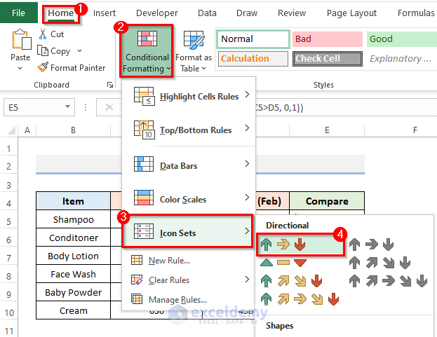
Now, we will use conditional formatting icon sets to visualize them. For this, at first, we will select the whole column E.
Subsequently, go to the Home tab from the ribbon.
Then, under the Styles group, click on the Conditional Formatting drop-down menu.
Go to Icon Sets options and select the Directional icons first option.

The icon is set in the column.

Suppose, we want to see the icons only, we don’t want the numbers of comparison. For this, select the column first.
Further, go to the Home tab from the ribbon.
Next, select the Conditional Formatting drop-down option from the Styles group.
Select the New Rule option.

This will display the New Formatting Rule dialog box.
Select Format all cells based on their values from Select a Rule Type.
Then, in the Edit the Rule Description dialog, we will edit all the necessary criteria.
Select Icon Sets from the Format Style drop-down menu.
Further, choose the Directional Icons from Icon Style drop-down option.
Checkmark the Show Icon Only option.
In the Values field, type 2 and 1, sequentially in the >= box.
Finally, to complete the process click on the OK button.

This will show only the icons.

Example 2: Compare Relative Row with Conditional Formatting Icon Sets Using Excel SIGN Function

In this example, we will employ the SIGN function to compare relative rows. This function returns the sign of an integer. When a positive number is entered, the SIGN function will output 1. The SIGN returns -1 if the value is negative.

To do this, we are going to use the dataset below. And the dataset has some months and units sell each month.

STEPS:

As shown in the earlier examples, firstly, select the cell and insert the formula into that cell.

=SIGN(C6-C5)

Press Enter to show the result in that selected cell.

After that, drag the Fill Handle down to copy the formula over the range. Or, double click on the plus (+) sign. This also duplicates the formula.

You can now see the result in the resulting column.

We will now visualize them using icon sets for conditional formatting. We shall first choose the entire column D for this.
Then, go to the ribbon and then, choose the Home tab.
Next, select the Conditional Formatting drop-down option from the Styles group.
Select the Directional icons first option under Icon Sets.

Thus, you will be able to see the Icon beside the result.

Let’s say we simply want to view the icons and don’t want the comparative figures. Choose the column first for this.
Go to the Home tab by selecting it from the ribbon.
Next, choose the Styles group’s Conditional Formatting drop-down option.
Choose Manage Rules from the menu.

Consequently, the Conditional Formatting Rules Manager dialog will appear.
Click on Edit Rule.

Therefore, the Edit Formatting Rule dialog will display.
Change the Values shown in the screenshot below and checkmark the Show Icon Only option.
Furthermore, click on OK.

This will take you again to the Conditional Formatting Rules Manager dialog.
Lastly, click on the OK button to complete the process.

Hence, you can see the icons only.

Things to Keep in Mind

Cell references in conditional formatting criteria are positioned in relation to the applicable range’s top-left cell. As a result, constantly including the first row of data when writing the conditional formatting.
Data may become more obvious with the aid of conditional formatting. To make advantage of it, construct rules that specify how cells should be formatted based on their values.

Download Practice Workbook

You can download the workbook and practice with them.

Icon Sets with Relative Reference.xlsx

Conclusion

The above examples will assist you to Use Excel Conditional Formatting Icon Sets with Relative Reference. Hope this will help you! Please let us know in the comment section if you have any questions, suggestions, or feedback.

<< Go Back to Icon Sets | Conditional Formatting | Learn Excel

Get FREE Advanced Excel Exercises with Solutions!