How to Change the Conditional Formatting Icon Set Color in Excel

Q: Does changing the Icon Set color affect the source data?

No, changing the Icon Set color doesn't impact the source data. It enhances the presentation without changing the data.

Q: Are there color limitations for Icon Sets?

There are no limitations. But it's recommended to select colors from the broad spectrum to maintain clarity and ensure easy interpretation of the icons.

Q: Will the custom Icon Set colors stay the same when I share the Excel file?

Yes, the customized Icon Set colors are saved within the Excel file, ensuring consistency when sharing the workbook with others.

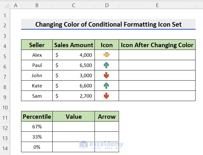
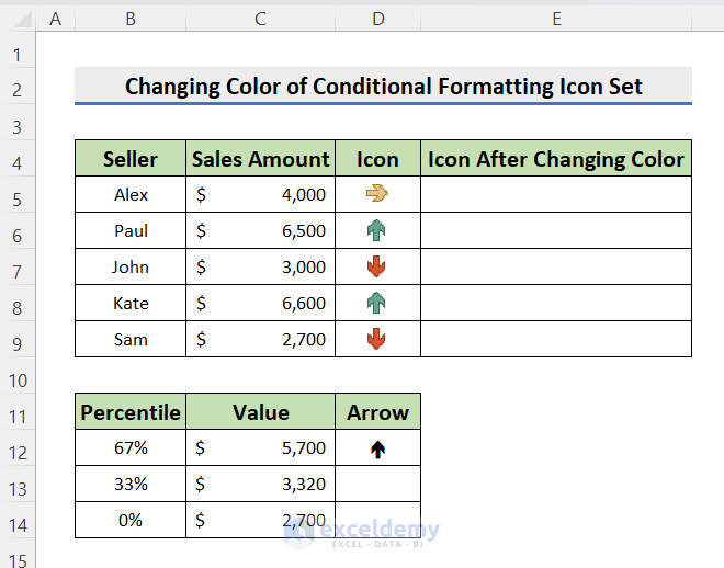
This is an overview. You can see the different colors of the icons in the columns “Before Changing” and “After Changing.”

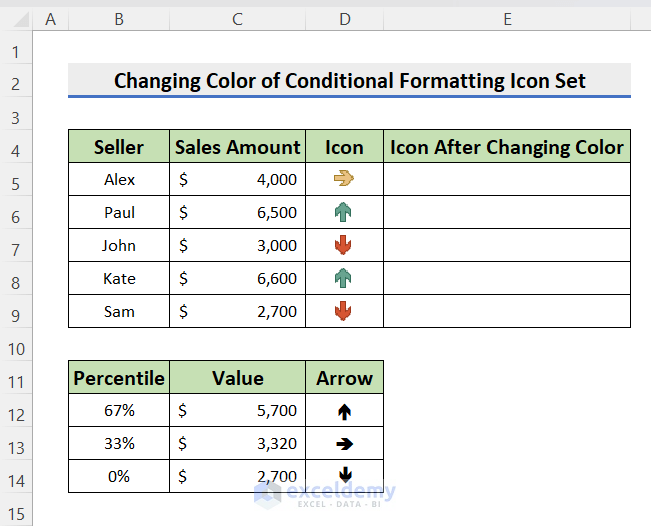
In the image below, you can see the Conditional Formatting Icon sets based on the percentage values using the Three Arrows (Colored) option. The Conditional Formatting Icon Sets divided the data range into three sections. A green up arrow appears when the relative cell value is above 67%, a yellow horizontal arrow for values between 33% and 67%, and a red down arrow for values below 33%.

The following conditions were considered to apply the conditional formatting icon sets.

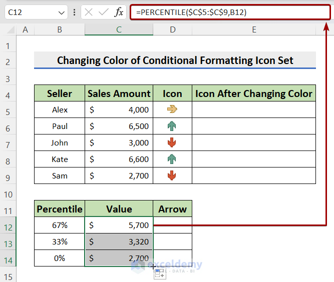
Step 1 – Create a Percentile Table

Use the PERCENTILE function.

Create a table with three columns including Percentile, Value, and Arrow.
In the Percentile column, enter 67%, 33%, and 0%.
Go to the first cell of the Value column.
Enter the following formula: =PERCENTILE($C$5:$C$9,B12)
Drag down the Fill Handle to see the output in the rest of the cells.

Step 2 – Insert Symbols

Go to Insert > Symbols > Symbol.
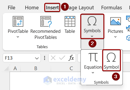
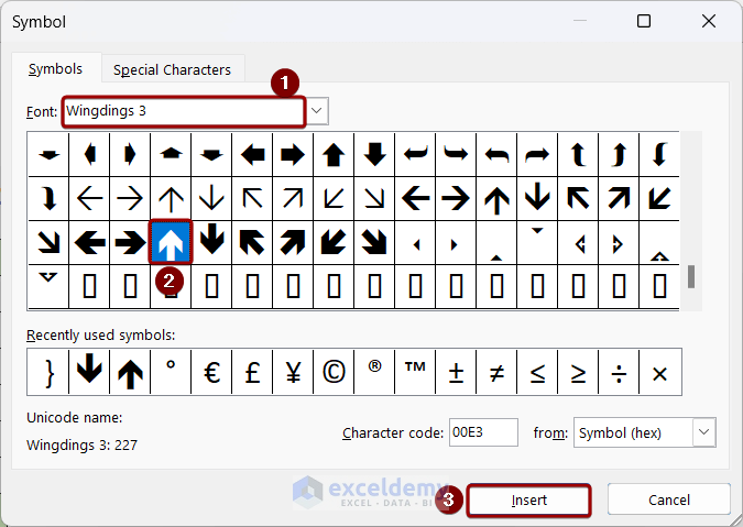
In the Symbol dialog box:
- Select Wingdings 3 in Font.
- Select the up arrow symbol and click Insert.
The symbol is inserted in the first cell of the percentile table.
Repeat the same process to insert horizontal and down arrows.

Step 3 – Use the IF Function to Set Icons

Use the IF function.

Enter the following formula in the first cell of the target column: =IF(C5="","",IF(C5>=$C$12,$D$12,IF(AND(C5>=$C$13,C5<$C$12),$D$13,$D$14)))
Press Enter and drag down the Fill Handle. 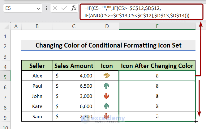Fonts are showing instead of arrows.
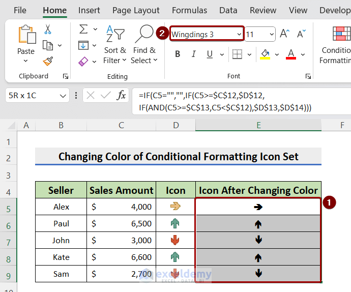
Select the data range of the output column.
Go to the Home tab > Font.
Choose Wingdings 3 in Font to see the arrows.

Step 4 – Change the Color of the Icon Sets

Select the data range containing icons.
Go to Home > Styles > Conditional Formatting > New Rule.
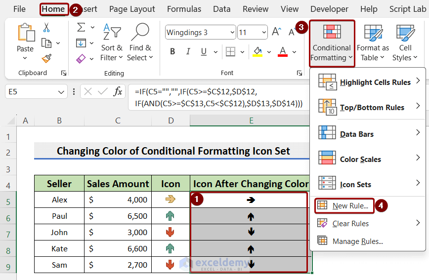
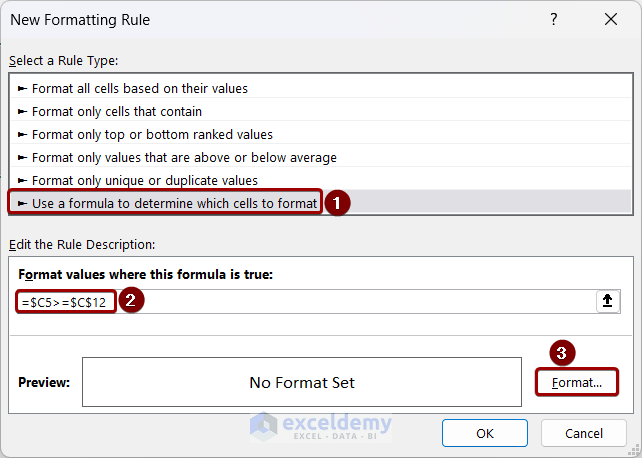
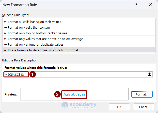
In the New Formatting Rule window:
- In Select a Rule Type > Use a formula to determine which cells to format.
- In “Format values where this formula is true:”, use the following formula: =$C5>=$C$12
- Click Format.
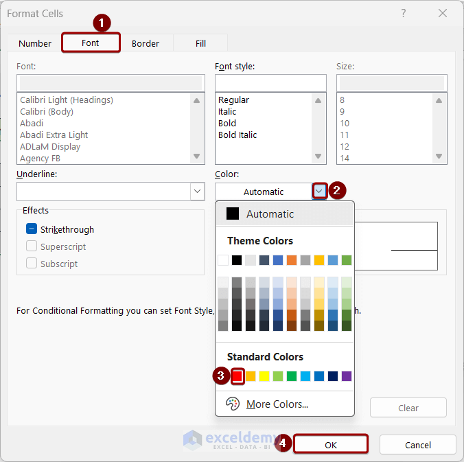
In the Format Cells dialog box:
- Go to the Font tab.
- Choose a color in Color.
- Click OK.
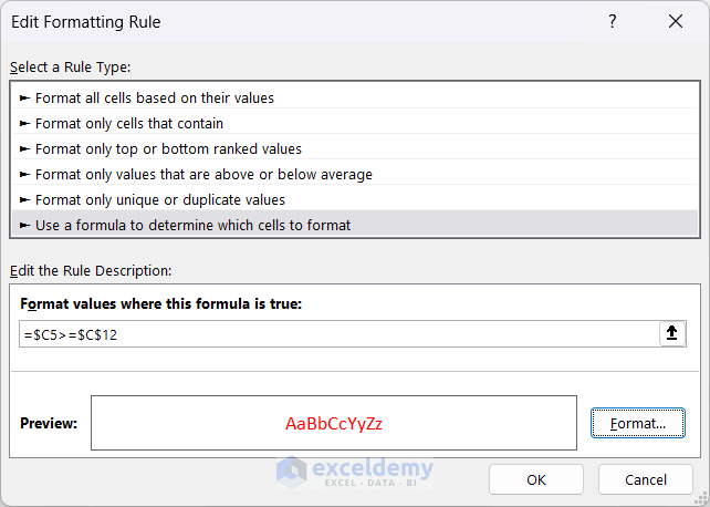
The New Formatting Rule window displays the preview.
Click OK. The color of the upward arrows changed.
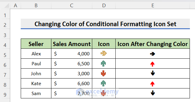
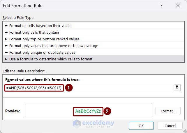
Repeat the process and enter the following formula: =AND($C5<$C$12,$C5>=$C$13)
Set another color for this rule and see the Preview.
Click OK.
Enter another formula as a rule: =$C5<$C$13
Set a different color for the rule and click OK.