While working with a big dataset in Excel that contains numerous entries, we need to find texts based on their specific text values, conditions, and duplicate or unique values. Conditional Formatting to color text is one of the convenient ways to highlight a cell’s text to make them identifiable immediately in Excel. In this article, we’ll demonstrate 3 convenient methods to do that properly.
Download the Practice Workbook
3 Easy Ways to Apply Conditional Formatting to Color Text in Excel
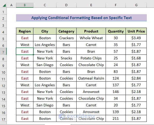
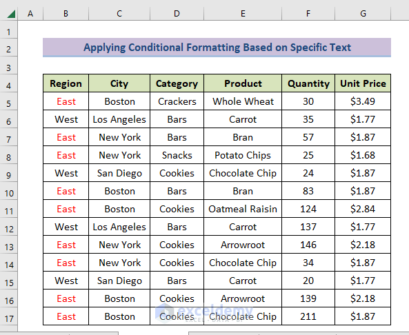
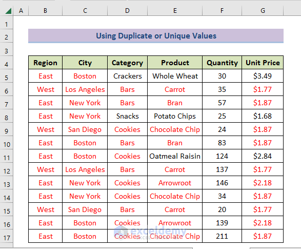
Suppose we have a Product Sales dataset containing text values such as Regions, Cities, Categories, and Products. We have multiple text values and want to conditionally format text color depending on the specific text. 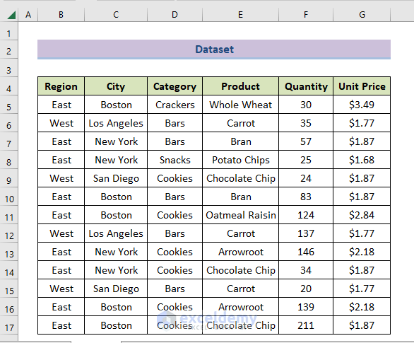
Method 1 – Applying Conditional Formatting to Color Text Based on Specific Text
Case 1 – Using the Text that Contains Option
Steps:
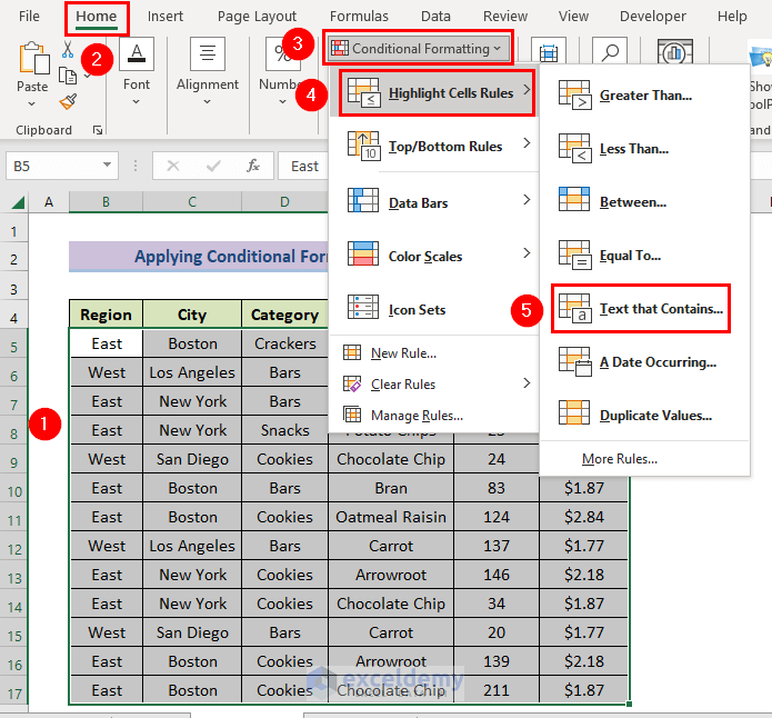
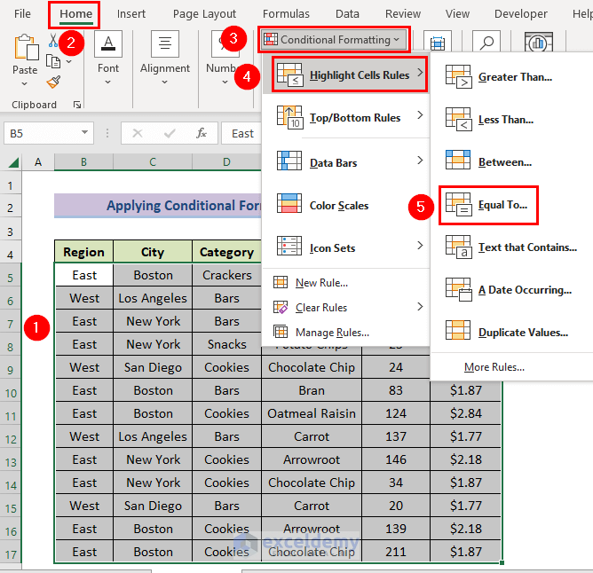
- Select the cells you want to conditionally format.
- Go to the Home Tab and select Conditional Formatting (from Styles section).
- Choose Highlight Cells Rules and select the Text that Contains option.
- The Text that Contains dialog box pops up. Type any existing text (i.e., East) in Format cells that contain the text box.
- Select Red Text in With section. You can choose different options to highlight text.
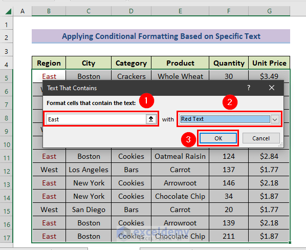
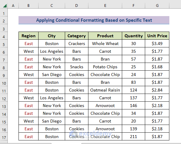
- You’ll discover all the strings that contain East get conditionally formatted with the selected text color similar to the following image.
Case 2 – Using the Equal to Option
Steps:
- Select a range of cells you want to format the text color.
- In the Home tab, go to Conditional Formatting (in the Styles section).
- Go to Highlight Cells Rules and select the Equal to option.
- Repeat Steps of Case 1 of Method 1, you’ll encounter all the specific text (i.e., East) formatted with text color as shown in the picture below.
Case 3 – Using the New Rule Option
Steps:
- Select a range of cells.
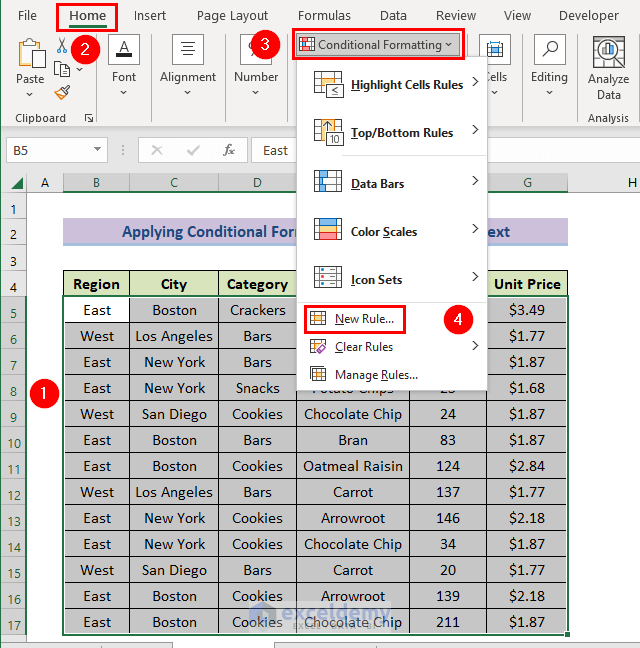
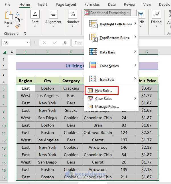
- Go to Home and select Conditional Formatting (in Styles section).
- Choose New Rule.
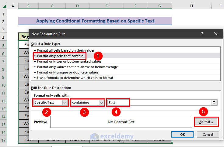
- The New Formatting Rule command window appears.
- Select Format only cells that contain as Select a Rule Type.
- Choose Specific Text and containing under the Format only cells with drop-down option box.
- Type the specific text (i.e., East).
- Click on Format.
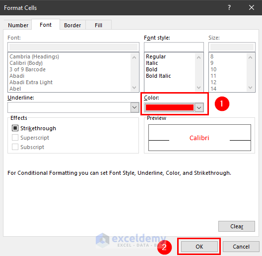
- In the Format Cells windown select Font color and press OK.
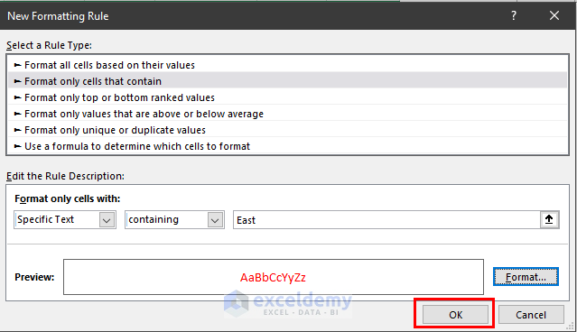
- You will return to the New Formatting Rule box. Click on OK.
- This returns a result similar to the image below.
Read More: Conditional Formatting Multiple Text Values in Excel (4 Easy Ways)
Method 2 – Using a Custom Rule to Conditionally Format Text Color
Steps:
- Select a range of cells then move to the Home tab and choose Conditional Formatting (in the Styles section).
- Select New Rule.
- You will see a New Formatting Rule window appear.
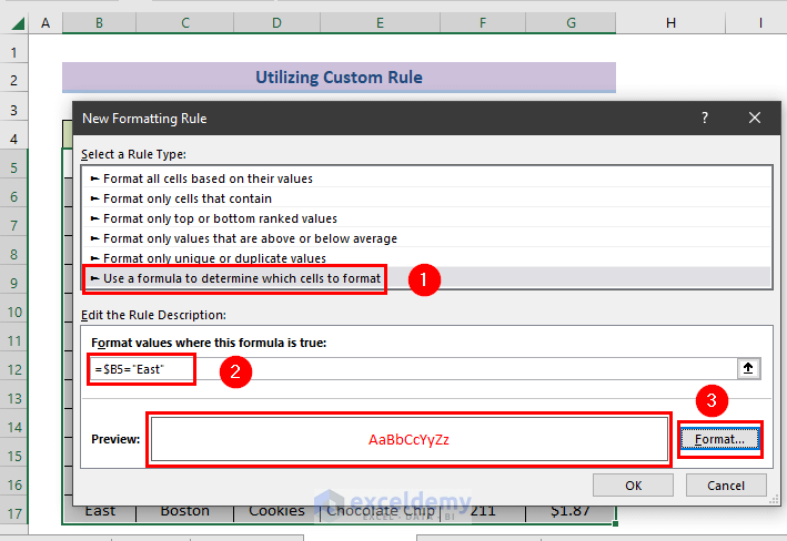
- Choose Use a formula to determine which cells to format as Select a Rule Type.
- Use the below formula in the Format values where this formula is true box.
=$B5="East"- The formula formats all the rows that contain “East” in Region Column (i.e., Column B)
- Click on Format.
- Follow the steps in Method 1, Case 3 to set the font color for highlighting.
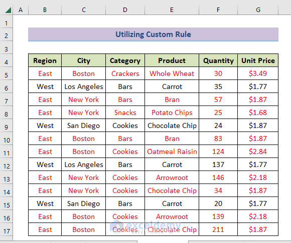
- You’ll get a similar result depicted in the image below.
Read More: How to Change Row Color Based on Text Value in Cell in Excel
Similar Readings
- How to Use Conditional Formatting Based on VLOOKUP in Excel
- Highlight Highest Value in Excel (3 Quick Ways)
- How to Highlight Lowest Value in Excel (11 Ways)
- Use Conditional Formatting in Excel Based on Dates
- Excel Conditional Formatting Dates Older than Today (3 Simple Ways)
Method 3 – Using Duplicate or Unique Values to Conditionally Format Text Color
Case 1 – Duplicate Values
Steps:
- Repeat the initial steps of Method 2.
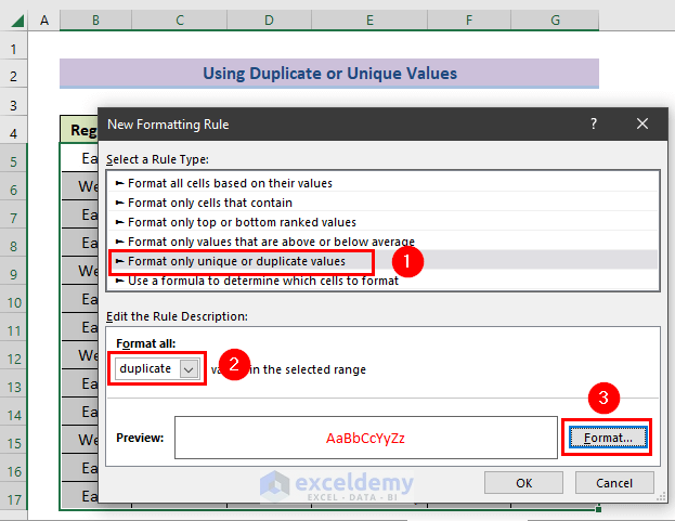
- Select Format only Unique or Duplicate Values as Select a Rule Type and choose duplicate under Format all box.
- Set the Format as in Method 1 Case 3.
- Click OK.
- All the duplicate values get formatted with the selected text color.
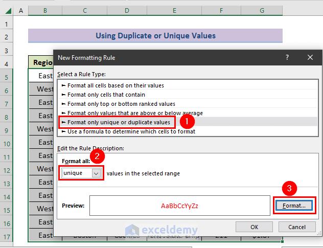
Case 2 – Unique Values
Steps:
- Follow the instructions derived in the initial steps of Case 1 in Method 3.
- Choose Unique in Format all box.
- Set the format as in steps of Method 1 Case 3.
- Click OK.
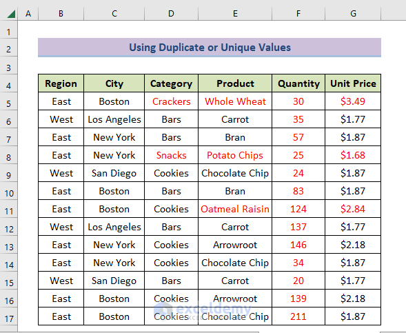
- This results in formatting all the unique cells in the range.
Read More: How to Use Conditional Formatting in Excel [Ultimate Guide]
Related Articles
- Excel Conditional Formatting Formula
- Conditional Formatting Dates
- How to Make Negative Numbers Red in Excel (4 Easy Ways)
- How to Compare Two Lists and Return Differences in Excel

