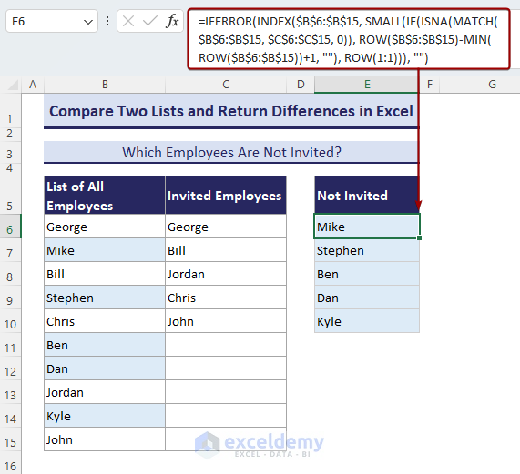
We have 2 lists: A list of all employees and a list of invited guests. We’ll compare the lists and see which employees were not invited. In the image below, you can see the missed employees who are not invited in column E.
Method 1 – Use a Formula with IF and COUNTIF to Compare 2 Lists and Return Differences in All Excel Versions
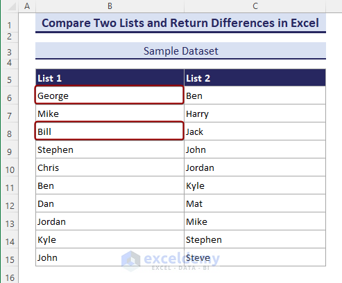
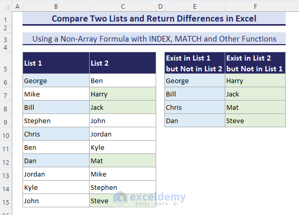
Let’s consider the following dataset. It contains two simple lists of some names.
Steps:
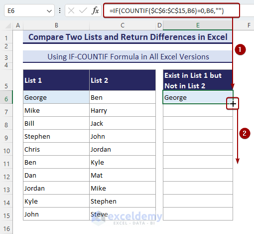
- Insert the following formula in the E6 cell and press Enter.
=IF(COUNTIF($C$6:$C$15,B6)=0,B6,"")- Copy this formula for the rest of the cells below. You will get the names that are in List-1 but not in List-2.
- By using the following formula in the F6 cell, you will get the names that are in List-2 but not in List-1.
=IF(COUNTIF($B$6:$B$15,C6)=0,C6,"")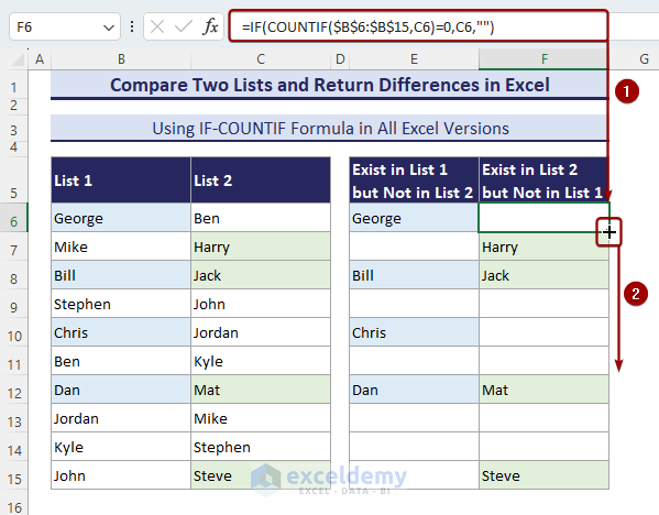
Method 2 – Use an INDEX-MATCH Formula to Get the Differences from 2 Columns (Non-Array Formula)
- When you enter this formula in a cell (here, in cell E6), it will return the first difference from List-1.
=INDEX($B$6:$B$15, SMALL(IF(ISNA(MATCH($B$6:$B$15, $C$6:$C$15, 0)), ROW($B$6:$B$15)-MIN(ROW($B$6:$B$15))+1, ""), ROW(1:1)))
- To get all the next differences, copy the formula down until it shows the #NUM! Error.
- If you don’t want to see those #NUM! error, use the following formula instead:
=IFERROR(INDEX($B$6:$B$15, SMALL(IF(ISNA(MATCH($B$6:$B$15, $C$6:$C$15, 0)), ROW($B$6:$B$15)-MIN(ROW($B$6:$B$15))+1, ""), ROW(1:1))), "")
- If you want to know which names are in List 2 but not in List 1, you can use the same formula with a few changes:
=IFERROR(INDEX($B$6:$B$15, SMALL(IF(ISNA(MATCH($B$6:$B$15, $C$6:$C$15, 0)), ROW($B$6:$B$15)-MIN(ROW($B$6:$B$15))+1, ""), ROW(1:1))), "")- Insert the formula above in cell F6 and drag the Fill handle tool to get all names in List 2 that do not exist in List 1.
Get Your Differences in A to Z Order
- You can use the following formula to get these differences in A to Z order.
=IFERROR(INDEX($B$6:$B$15,MATCH(SMALL(IF((COUNTIF($E$5:E5,$B$6:$B$15)+COUNTIF($C$6:$C$15,$B$6:$B$15))=0,COUNTIF($B$6:$B$15,"<"&$B$6:$B$15)),1),COUNTIF($B$6:$B$15,"<"&$B$6:$B$15),0)),"")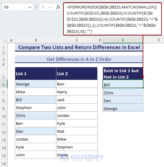
Read More: Excel formula to compare two columns and return a value
Method 3 – Use IF, ISNA, and MATCH Functions to Compare and Get Differences from 2 Columns with an Array Formula
- Put this formula in a cell (cell E6):
=IF(ISNA(MATCH($B$6:$B$15, $C$6:$C$15, 0)), $B$6:$B$15, "")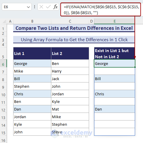
- This is an array formula and hence it will display #SPILL! error when merged or non-blank cells exist in E6:E15 or F6:F15.
- This formula can’t return all the differences together in adjacent cells. To solve this, you can add the SORT function with this formula if you have Excel 2021 or 365.
=SORT(IF(ISNA(MATCH($B$6:$B$15, $C$6:$C$15, 0)), $B$6:$B$15, ""),1,-1)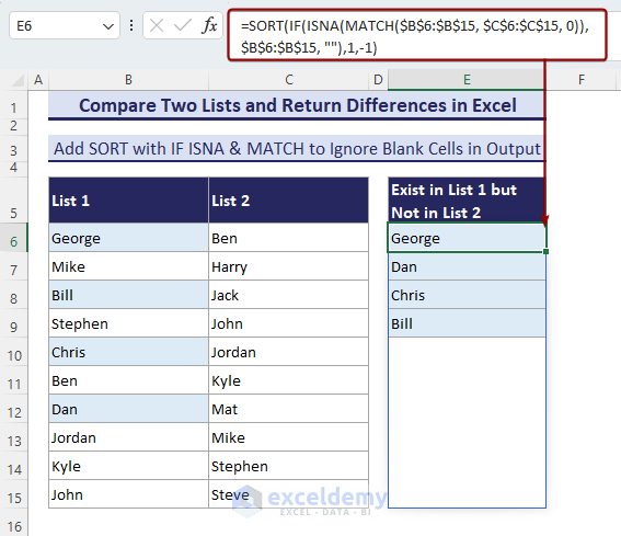
Method 4 – Combine TEXTJOIN with an IF-ISNA-MATCH Formula to Get All Unmatched Values in a Single Cell
- Use the following formula in the E6 cell and press Enter.
=TEXTJOIN(", ", TRUE, IF(ISNA(MATCH($B$6:$B$15, $C$6:$C$15, 0)), $B$6:$B$15, ""))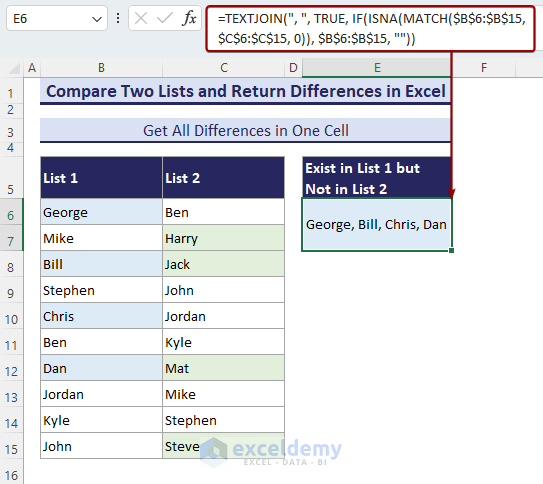
Method 5 – Use FILTER and COUNTIF Functions in Excel 2019 or Later Versions
- Apply the formula as follows in the E6 cell and hit Enter.
=FILTER(B6:B15,COUNTIF(C6:C15,B6:B15)=0)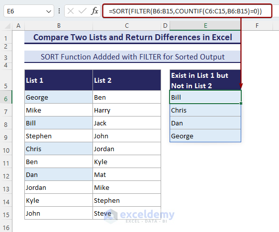
Method 6 – Use VBA Code to Compare Two Lists and Return Differences
The VBA code in this section is applicable to any two lists.
- Copy the VBA code in the module and save the Macro.
Sub Compare_Two_Lists_and_Return_Differences()
‘Developed by MD_Tanvir_Rahman, ExcelDemy
Dim rng As Range
Dim Output_rng As Range
Dim i As Integer
Dim j As Integer
Dim outputRow1 As Integer
Dim outputRow2 As Integer
Set rng = Application.InputBox("Select Input Range:", Type:=8)
Set Output_rng = Application.InputBox("Select Output Range:", Type:=8)
outputRow1 = 1
outputRow2 = 1
For i = 1 To rng.Rows.Count
    Dim foundMatch1 As Boolean
    foundMatch = False
    For j = 1 To rng.Rows.Count
        If rng.Cells(i, 1).Value = rng.Cells(j, 2).Value Then
            foundMatch = True
            Exit For
        End If
    Next j
    If Not foundMatch Then
        Output_rng.Cells(outputRow1, 1).Value = rng.Cells(i, 1).Value
        outputRow1 = outputRow1 + 1
    End If
Next i
For i = 1 To rng.Rows.Count
    Dim foundMatch2 As Boolean
    foundMatch = False
    For j = 1 To rng.Rows.Count
        If rng.Cells(i, 2).Value = rng.Cells(j, 1).Value Then
            foundMatch = True
            Exit For
        End If
    Next j
    If Not foundMatch Then
        Output_rng.Cells(outputRow2, 2).Value = rng.Cells(i, 2).Value
        outputRow2 = outputRow2 + 1
    End If
Next i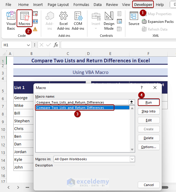
End Sub- Go to Developer and select Macros.
- Select Compare_Two_Lists_and_Return_Differences and hit Run.
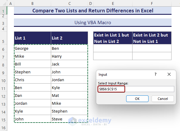
- An Input dialog box shows up. Select the $B$6:$C$15 range and click OK.
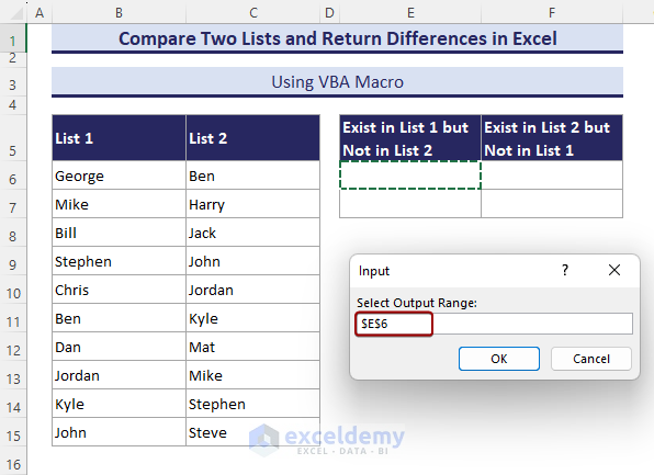
- Another Input dialog box shows up. Select the $E$6 range and click OK.
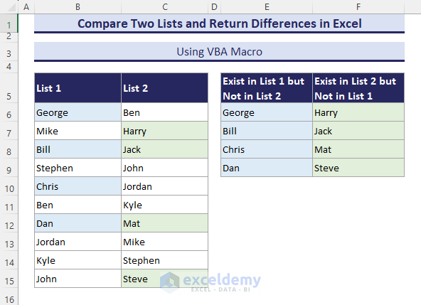
- We obtain all the differences of both lists in the E6:F9 range.
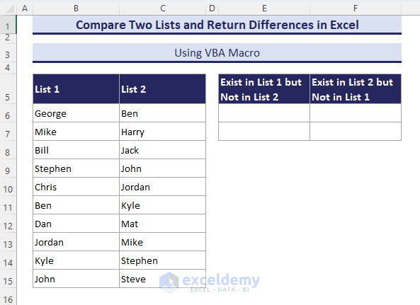
- The VBA Macro doesn’t update data automatically. You must Run the macro every time the data changes.
- We used Conditional Formatting to highlight the differences, not the statements inside VBA Macro.
How to Create a Dynamic Formula That Compares 2 Columns and Returns Differences When You Add New Items
Method 1
- Use the following formula:
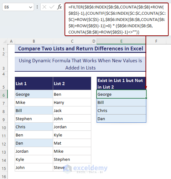
=FILTER($B$6:INDEX($B:$B,COUNTA($B:$B)+ROW($B$5)-1),(COUNTIF($C$6:INDEX($C:$C,COUNTA($C:$C)+ROW($C$5)-1),$B$6:INDEX($B:$B,COUNTA($B:$B)+ROW($B$5)-1))=0)*($B$6:INDEX($B:$B,COUNTA($B:$B)+ROW($B$5)-1)<>""))- If you use this formula in cell E6, you can add new items in the lists.
Method 2
- We will use the Named Range for the dynamic ranges.
- Go to Formulas tab and select Define Name.
- You’ll get a New Name dialog box.
- In the Refers to field, use the following:
='2.2 Dynamic (Named_Range)'!$B$6:INDEX('2.2 Dynamic (Named_Range)'!$B:$B,COUNTA('2.2 Dynamic (Named_Range)'!$B:$B)+ROW('2.2 Dynamic (Named_Range)'!$B$5)-1)- Name it as List_1.
- Click OK.
- Replace “2.2 Dynamic (Named_Range)” with your respective sheet name. Or, when you select the ranges, this will be automatically selected.
- You must add an underscore between words while naming formulas. Also, Press F2 if you want to edit anything in the Refers to field.
- Name the second list using the following formula and name it List_2.
='2.2 Dynamic (Named_Range)'!$C$6:INDEX('2.2 Dynamic (Named_Range)'!$C:$C,COUNTA('2.2 Dynamic (Named_Range)'!$C:$C)+ROW('2.2 Dynamic (Named_Range)'!$C$5)-1)- The formula will look like this.
=FILTER(List_1,(COUNTIF(List_2,List_1)=0)*(List_1<>""))
- Add a new name in List-1 and see what happens.
How to Compare Two Datasets with Multiple Columns and Return Whole Rows for Differences
We have two separate datasets such as the Current List and the New List. We need to find the mismatched data of the New List and gather differences of multiple Excel columns.
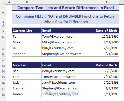
- Input the following formula in B21 and hit Enter.
=FILTER(B14:D18,(NOT(ISNUMBER(XMATCH(B14:B18,B6:B9)))*(B14:B18<>"")))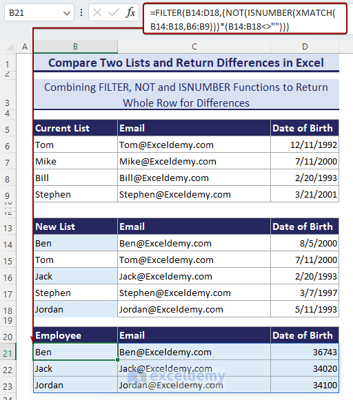
How to Compare Two Lists and Highlight Differences with Excel Conditional Formatting
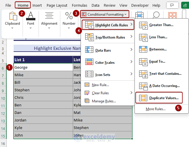
Method 1 – Use Highlight Cell Rules to Mark Differences
- Select the range B6:C15 and go to Conditional Formatting, then go to Highlight Cells Rules and select Duplicate Values.
- The Duplicate Values dialog box shows up. Select Unique and click OK.
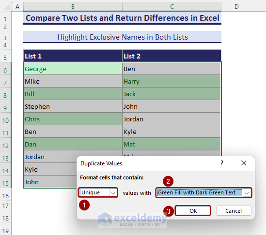
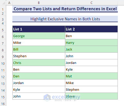
- All the unique names between List-1 and List-2 get highlighted.
Method 2 – Mark Differences with New Formatting Rule
- Select the range B6:B15 and go to Home, then to Conditional Formatting, and select New Rule.
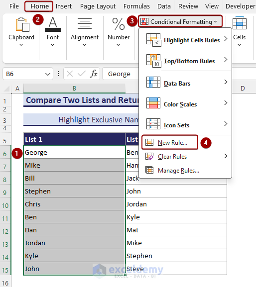
- The New Formatting Rule dialog box appears.
- Select Use a formula to determine which cells to format option from Select a Rule Type
- Insert the following formula in the formula box and click OK.
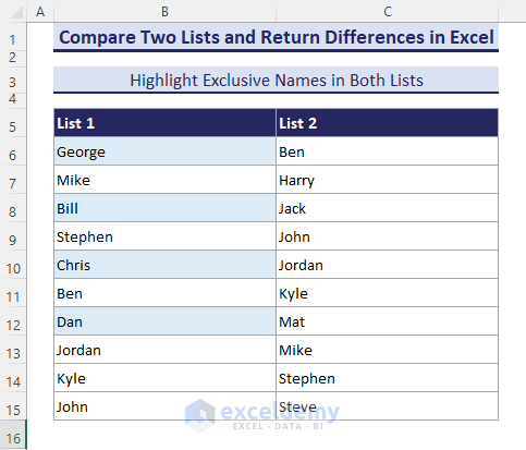
=COUNTIF($C$6:$C$15, B6) = 0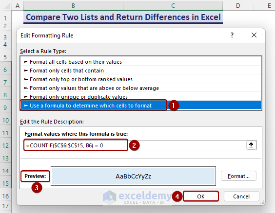
- All the unique values are highlighted in List-1.
- Selecting the C6:C15 range and applying the following formula highlights the unmatched names of List-2.
=COUNTIF($B$6:$B$15, C6) = 0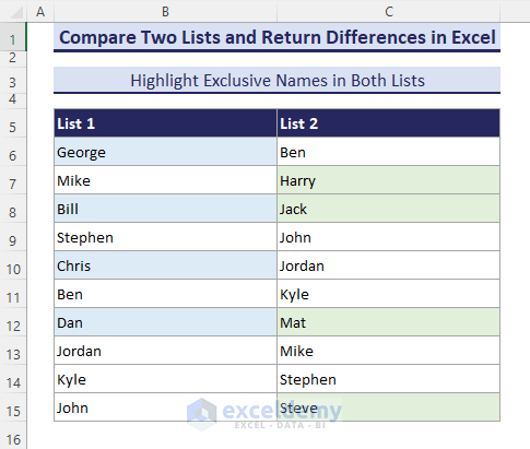
Download the Practice Workbooks
<< Go Back to Columns | Compare | Learn Excel
Get FREE Advanced Excel Exercises with Solutions!
