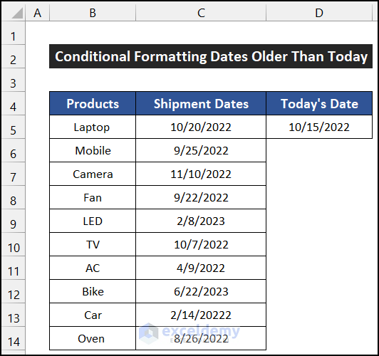
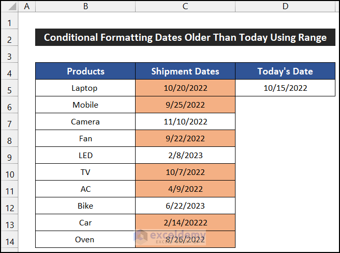
Let’s consider a shipment date of 10 items. The name of the items is in column B, their delivery time is in column C. So, our dataset is in the range of cells B5:C14. We get today’s date in cell D5 using the TODAY function.
The TODAY function will change the date automatically when you open the file on your device. The images in this article may not match your result.
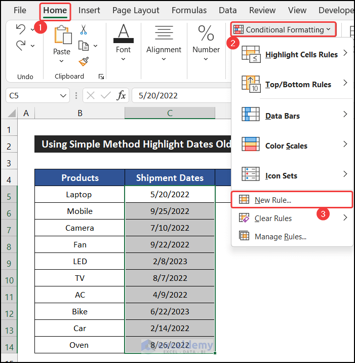
Method 1 – Apply Simple Conditional Formatting to Highlight Dates Older Than Today
Steps:
- Select the range of cells C5:C14.
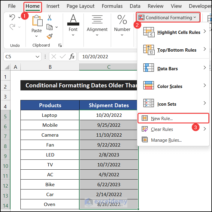
- In the Home tab, click on the drop-down arrow of the Conditional Formatting option from the Styles group and choose the New Rules option.
- A small dialog box called the New Formatting Rule will appear.
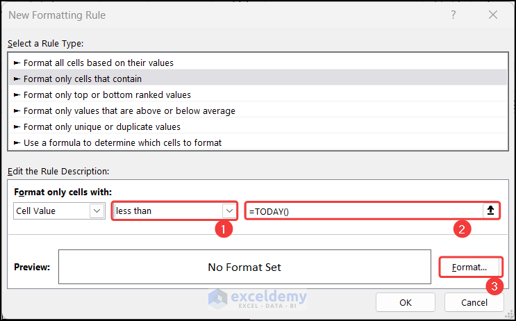
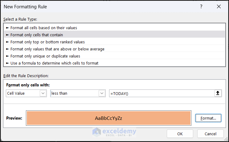
- Select the Format only cells that contain option.
- In the second field, change the option from between to less than.

- In the next empty field, copy the following formula:
=TODAY()
- Click the Format button.
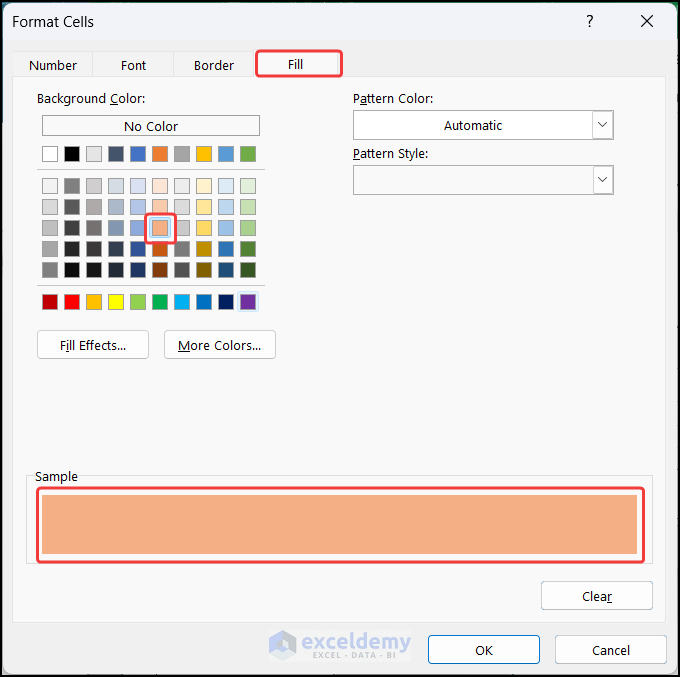
- Another dialog box called Format Cells will appear.
- In the Fill tab, choose a cell color. We chose Orange, Accent 2, Lighter 40% color.
- Click OK to close the dialog box.
- Click OK to close the New Formatting Rule dialog box.
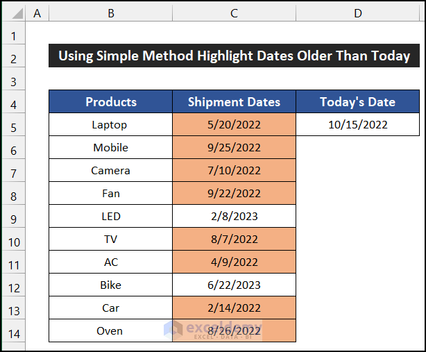
- You will see the dates which are older than today will get our desired cell color.
Read More: Highlight Row with Conditional Formatting Based On Date in Excel
Method 2 – Apply Conditional Formatting for Dates Older Than Today Using a Range
Steps:
- Select the range of cells C5:C14.
- In the Home tab, click on the drop-down arrow of the Conditional Formatting option from the Styles group and choose the New Rules option.
- A small dialog box called the New Formatting Rule will appear.
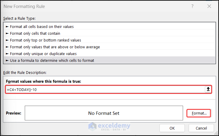
- Select the Use a formula to determine which cells to format option.
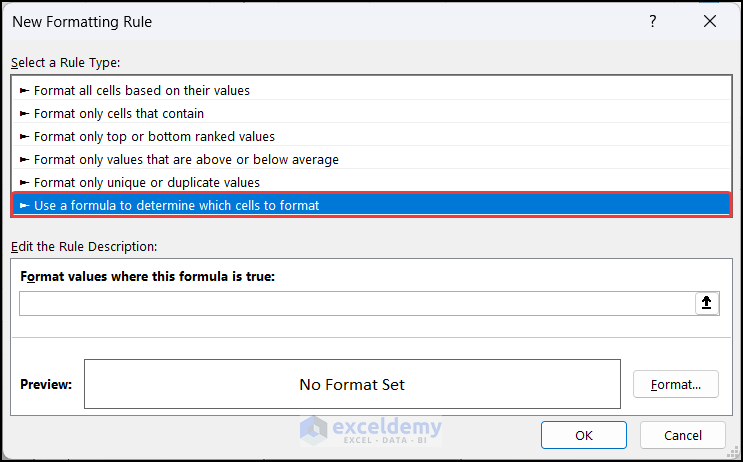
- In the empty field below the text Format values where this formula is true, copy the following formula:
=C4>TODAY()-10
- Click the Format button.
- Choose a Fill color from the selector.
- Click OK.
- Click OK to close the New Formatting Rule dialog box.

- The dates which are older than 10 days from today are now highlighted.
Read More: Excel Conditional Formatting Based on Date
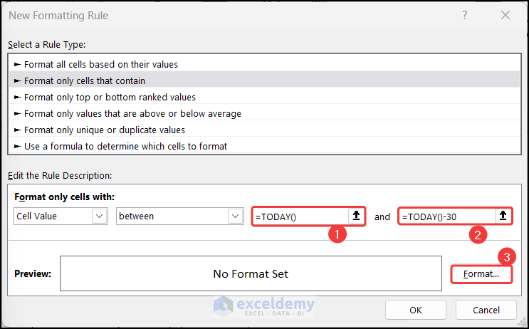
Method 3 – Highlight Dates Using Conditional Formatting Between Today and 30 Days Ago (Range of Dates)
Steps:
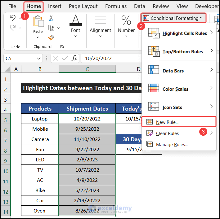
- Select the range of cells C5:C14.
- In the Home tab, click on the drop-down arrow of the Conditional Formatting option from the Styles group and choose the New Rules option.
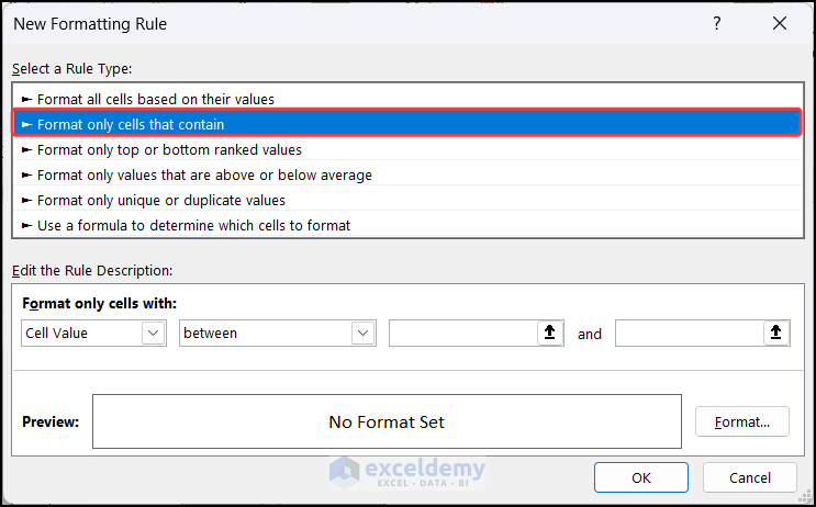
- A small dialog box called the New Formatting Rule will appear.
- Select the Format only cells that contain option.
- In the third empty box, copy the following:
=TODAY()
- In the remaining empty box, insert the following formula:
=TODAY()-30
- Click the Format button.
- Choose a color from the Fill tab.
- Click OK to close the Format cells dialog box.
- Click OK to close the New Formatting Rule dialog box.
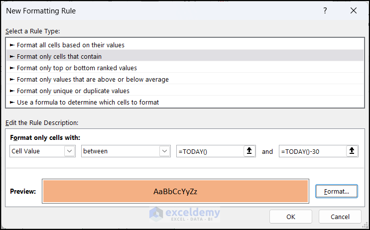
- Excel will highlight dates that are between today and 30 days ago.

Read More: How to Change Cell Color Based on Date Using Excel Formula
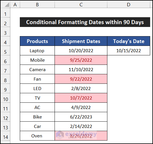
Apply Conditional Formatting for Dates within 90 Days
Steps:
- Select the range of cells C5:C14.
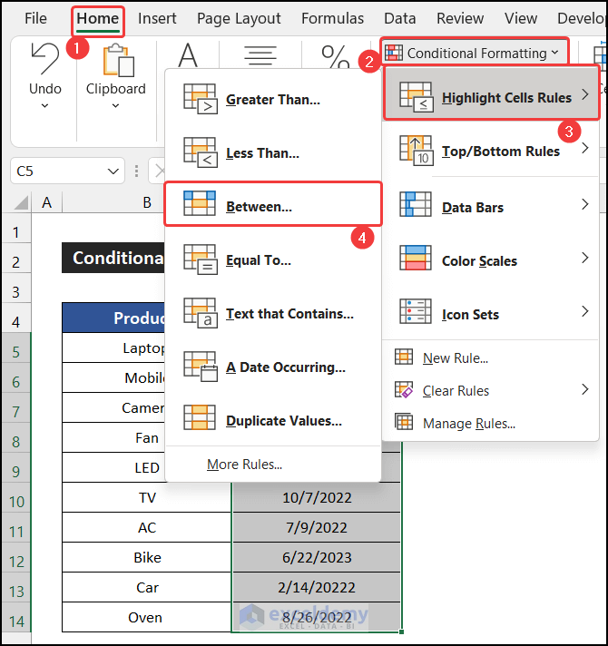
- In the Home tab, click on the drop-down arrow of the Conditional Formatting option from the Styles group.
- Select Highlight Cell Rules and choose the Between option.
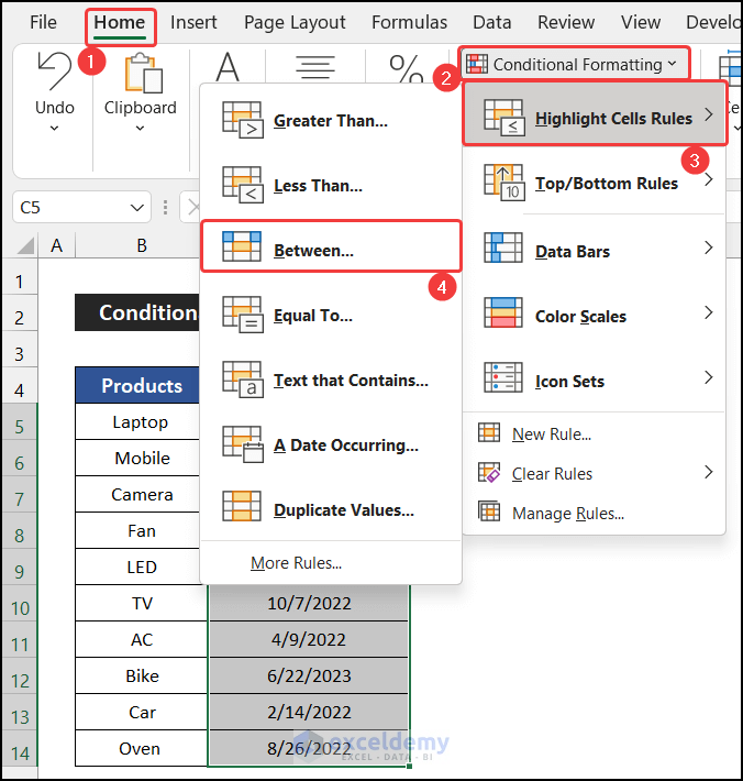
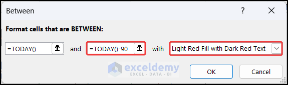
- A small dialog box called Between will appear.
- In the first box, remove the default date and insert the following formula:
=TODAY()
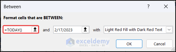
- In the next value box, copy the following formula:
=TODAY()-90
- If you want your custom format, select the Custom Format option from the drop-down arrow and create your custom formatting.
- Click OK to close the dialog box.
- Excel will highlight dates no older than 90 days ago.
Read More: Excel Conditional Formatting for Dates within 30 Days
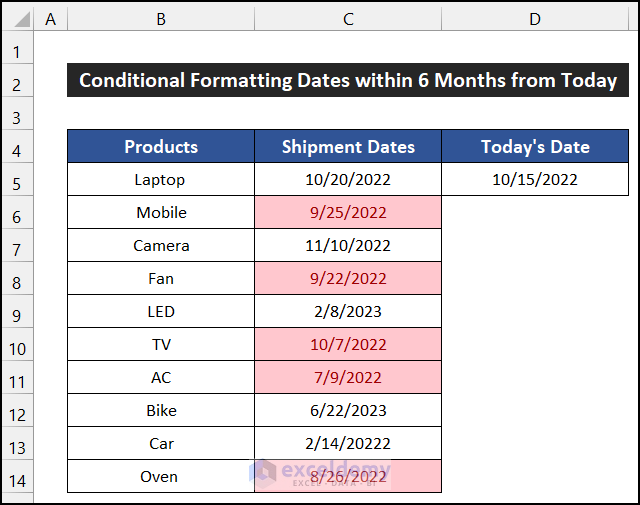
Perform Conditional Formatting for Dates Within 6 Months from Today
Steps:
- Select the range of cells C5:C14.
- In the Home tab, click on the drop-down arrow of the Conditional Formatting option from the Styles group.
- Select Highlight Cell Rules and choose the Between option.
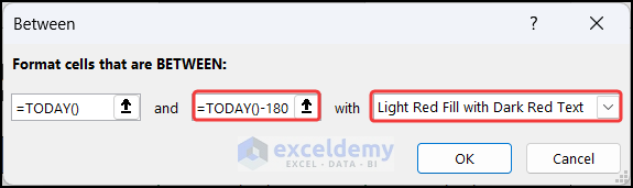
- A small dialog box called Between will appear.
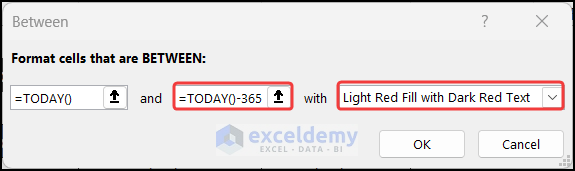
- In the first value box, remove the default date and insert the following:
=TODAY()
- In the second value box, insert the following:
=TODAY()-180
- Customize the format if you want by clicking the third box.
- Click OK to close the dialog box.
- You will get the dates with the default highlighting color.
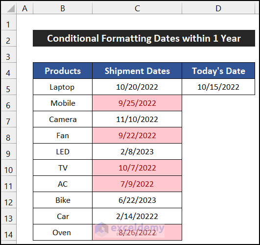
Use Conditional Formatting for Dates Within 1 Year
Steps:
- Select the range of cells C5:C14.
- In the Home tab, click on the drop-down arrow of the Conditional Formatting option from the Styles group.
- Select Highlight Cell Rules and pick the Between option.
- A small dialog box called Between will appear.
- In the first value box, remove the default date and insert the following:
=TODAY()
- In the second box, insert the following:
=TODAY()-365
- Customize the format in the third box if you want.
- Click OK to apply the formatting.
- You will get the dates with the chosen highlighting color.
Download Practice Workbook
Download this workbook for practice. Modify the dates to check if the highlighting works.
Related Articles
- Conditional Formatting Based on Date in Another Cell in Excel
- Apply Conditional Formatting to Overdue Dates in Excel
- How to Apply Conditional Formatting to Each Row Individually
- How to Apply Conditional Formatting to Multiple Rows
- Conditional Formatting on Multiple Rows Independently in Excel
- How to Change Row Color Based on Text Value in Cell in Excel
<< Go Back to Conditional Formatting Based on Date | Conditional Formatting | Learn Excel
Get FREE Advanced Excel Exercises with Solutions!

Very clear instructions. How to make it so the blanks don’t get filled in?
Hello, JACK! For this, you have to add a new conditional Formatting rule. Go to Home tab >> Conditional Formatting >> New Rule.
Then, Select the “Format Only Cells That Contain” and select the “Blanks” option in the “Format only cells with” box.
Then, go to the “Format” option and select White as the fill color.
Try this and let us know the outcome. Thank you!
Is there a way to apply this rule so that the entire row is highlighted instead of just the cell?
Hello Noelle,
To highlight the entire row, insert the following formula: =$C5 < TODAY()
In applies to select the rows
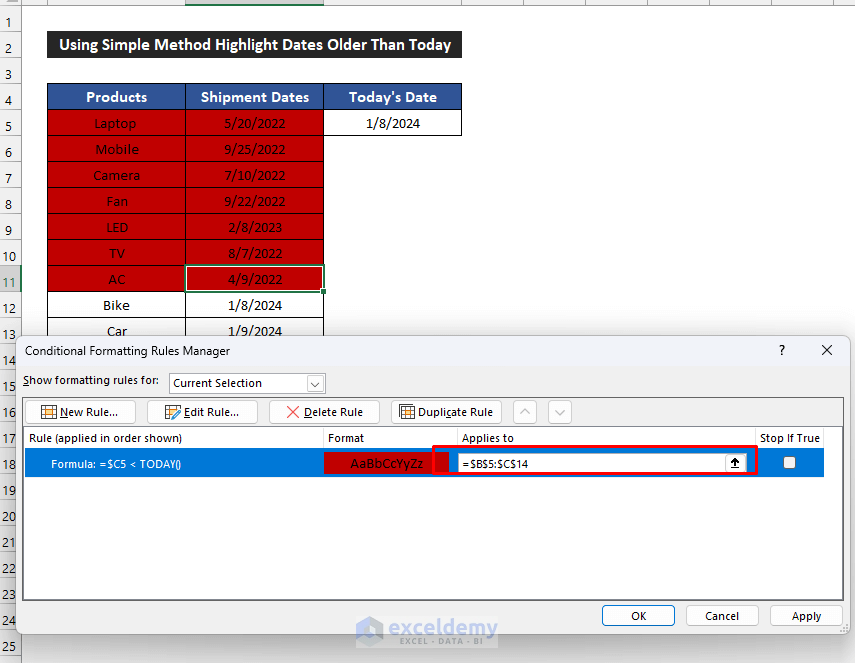
Regards
ExcelDemy
I need a future date alert. Most employees have taken a class on 3/1/2025 (others past that date). I don’t want to use =today()-whatever because the way I see it, if I place -70 then that will be the hard minus the next time they take the next class. That will not work because the class is renewed once a year. I need the countdown to start on 3/1/25 and alert me two months before 3/1/26 (1/1/26) to take the class again (this will apply for future years to come). Also, there are blank cells for new employees that have not taken a class which needs to alert me immediately. How do I create a condition for both? All this in column L2 to end.
Hello Ann,
You can do this with 3 Conditional Formatting rules on L2:L that “roll” every year using EDATE (no hard −70).
Applies to: =$L$2:$L$1000 (adjust as needed).
Set rule order as shown (use “Stop If True” where available):
Missing date → alert immediately
Formula: =ISBLANK($L2)
Overdue (past the 1-year mark)
Formula: =AND($L2<>“”, TODAY()>EDATE($L2,12))
Due soon (within 2 months of the next anniversary)
Formula: =AND($L2<>“”, TODAY()>=EDATE($L2,10), TODAY()<=EDATE($L2,12))
Why this works:
EDATE($L2,12) = the next renewal date (one year after the last class).
EDATE($L2,10) = two months before that date. For example, if L2 is 3/1/2025, then two-months-prior is 1/1/2026, which matches your target.
Give each rule a different fill color (e.g., red = overdue, amber = due soon, gray = missing). No helper columns needed, and it will keep working for future years automatically.
Regards,
ExcelDemy