How to Change Cell Color Based on Date Using Excel Formula

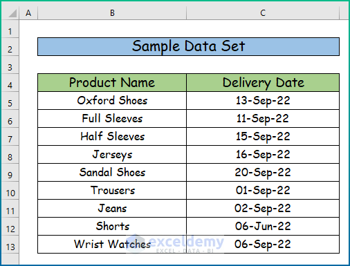
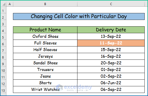
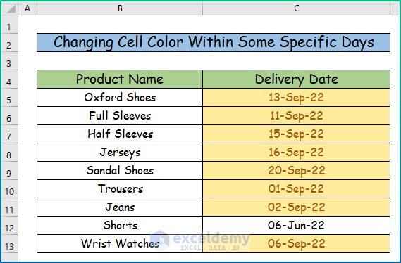
We will use the following sample data set to demonstrate how to change the color of a cell based on the date.

Method 1 – Change the Cell Color of Dates Based on Another Value

Case 1.1 – Greater Than Particular Date

Steps:

• Select the cell range C5:C13 and go to the Home tab of the ribbon.
• Under the Styles group, select Conditional Formatting.

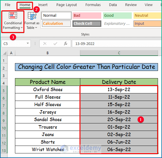
• Select Highlight Cells Rules and choose Greater Than.

• Enter the specific date with which you want to compare and choose the highlighting style.
• Press OK.

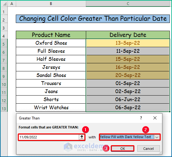
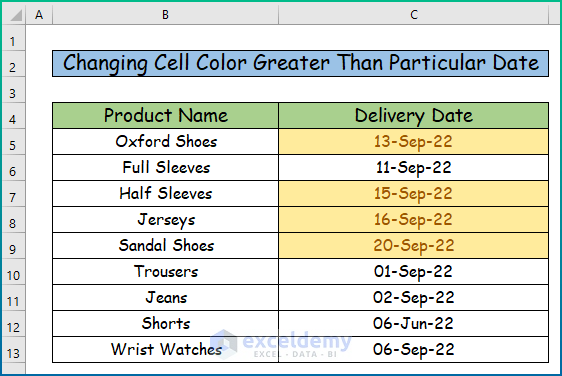
• The cells containing dates greater than the date in the Conditional Formatting Rule will change their colors.

Case 1.2 – Less Than Particular Date

Steps:

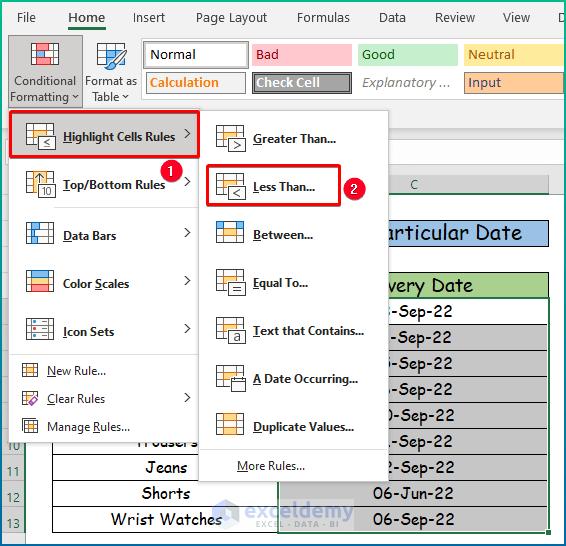
• Go to Conditional Formatting after choosing the cell range for highlighting.
• From the Highlight Cells Rules drop-down, select Less Than.

• Insert the date in the Less Than dialog box for comparison and specify the cell style after highlighting.
• Press OK.

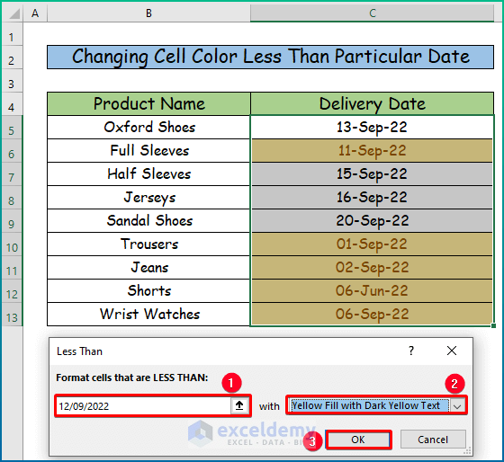
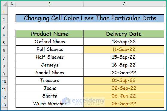
• Here’s the result for our sample and the date September 12, 2022.

Read More: Highlighting Row with Conditional Formatting Based on Date in Excel

Method 2 – Change Cell Color of Dates Between Two Particular Dates

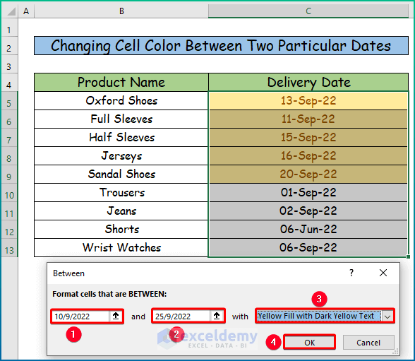
We want to change the colors of cells that contain dates between 10 September and 25 September 2022 to yellow.

Steps:

• Select the cell range C5:C17.

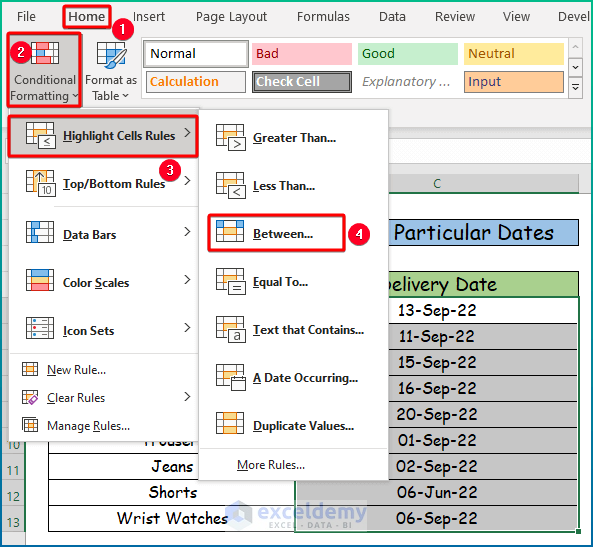
• Select Conditional Formatting from the Home tab of the ribbon.
• From the Highlight Cells Rules drop-down, select Between.

• In the Format cells that are BETWEEN option, insert the starting and ending date.
• Click the drop-down menu with and select the format you like.
• Click OK.

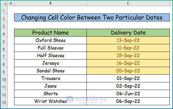
• Here’s the result for our sample.

Read More: Excel Conditional Formatting Based on Date

Method 3 – Change the Cell Color of Dates with a Particular Day

We want to change the cell colors that contain dates that fall on a Sunday.

Steps:

• Select the cell range and go to the Home tab of the ribbon.
• From the drop-down, select New Rule.

• Under the Select a Rule Type menu, click on the last option: Use a formula to determine which cells to format.
• In the Format values where this formula is true box, insert the following formula:

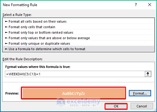
• Press Format to select the cell color and font style.

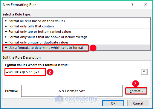
• After setting all the criteria, press OK in the dialog box.

• The dates that represents Sunday will be highlighted.

Read More: Conditional Formatting Based on Date in Another Cell in Excel

Method 4 – Change the Cell Color of Dates Within a Specific Period Before Today

Steps:

• Select the dates from cell range C5:C17 and go to the Home tab of the ribbon.
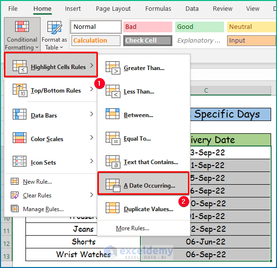
• Select the Conditional Formatting option under the Styles section.
• Select Highlight Cell Rules.
• Choose the A Date Occurring option.

• You will see the A Date Occurring dialog box.
• Click on the left drop-down menu and you will get multiple options.

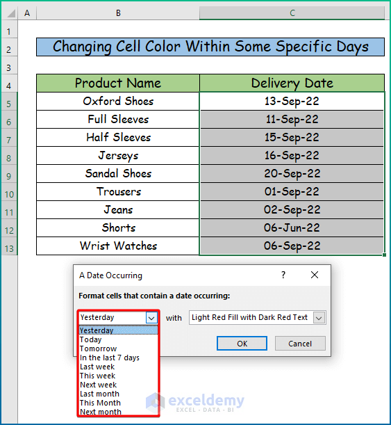
• Select an option. We want all the days within the last month to be highlighted, so we chose the Last month option.
• Specify the style criteria and press OK.

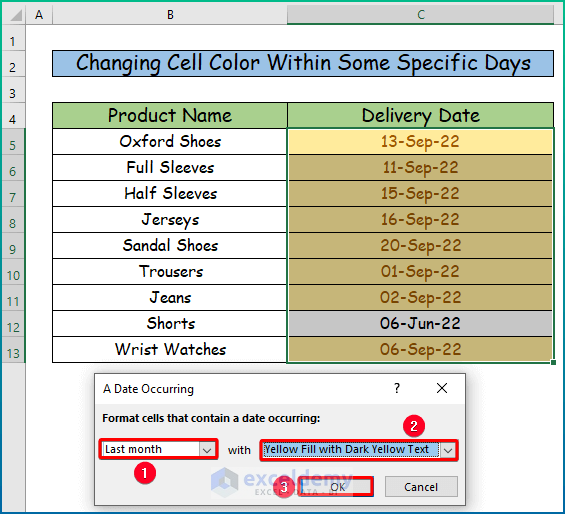
• Here’s our result.

Read More: Apply Conditional Formatting for Dates Older Than Today in Excel

Download the Practice Workbook

Related Articles

• Apply Conditional Formatting to Overdue Dates in Excel
• Excel Conditional Formatting for Dates within 30 Days
• How to Apply Conditional Formatting to Each Row Individually
• How to Apply Conditional Formatting to Multiple Rows
• Conditional Formatting on Multiple Rows Independently in Excel
• How to Change Row Color Based on Text Value in Cell in Excel

<< Go Back to Conditional Formatting Based on Date | Conditional Formatting | Learn Excel