Apply Conditional Formatting to Overdue Dates in Excel (3 Ways)

In this article, we will be using a project deadline list as a dataset to demonstrate all the methods.

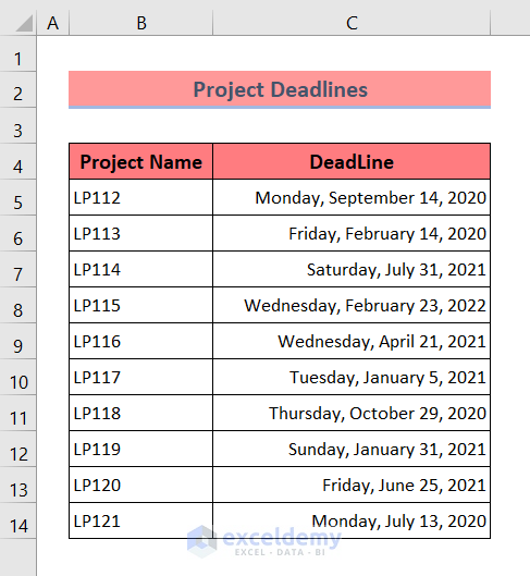
Method 1 – Apply Conditional Formatting to the Overdue Dates Using Less Than Command in Excel

Suppose you want to highlight all the cells containing dates before a specific date.

Steps:

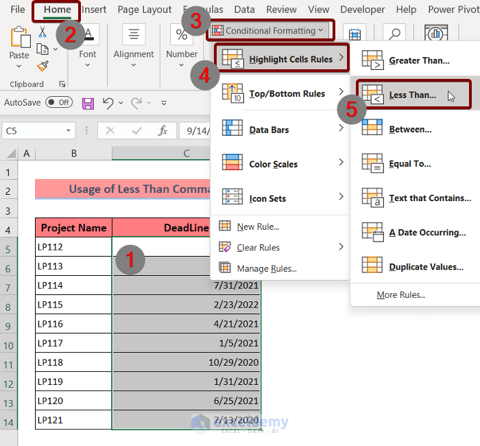
• Select the range of cells where you want to apply the formatting.
• Go to Home and select Conditional Formatting.
• Choose Highlight Cells Rules, then Less Than.

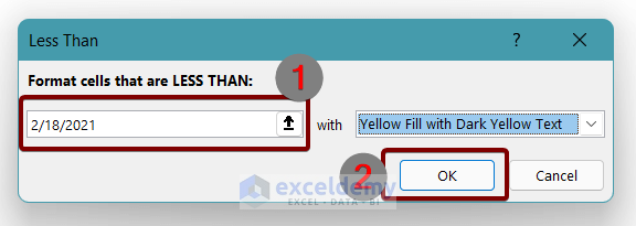
• The Less Than dialog box will appear. In the box, insert a date based on which all the cells containing dates before it will be highlighted with color.
• For instance, we’ve inserted the date 2/18/2021.
• Hit the OK button.

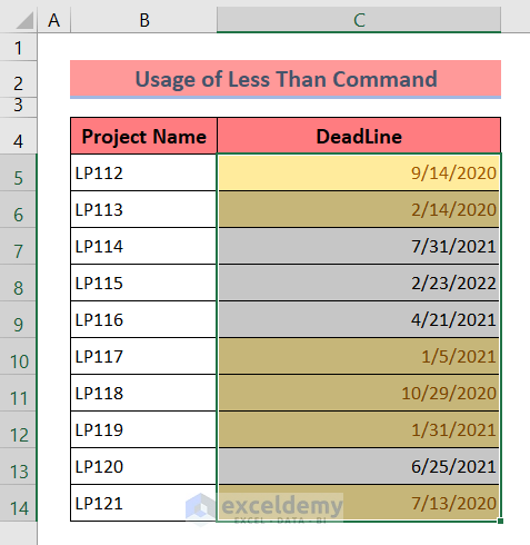
• You will get cells highlighted with color as in the image below:

Read more: Apply Conditional Formatting for Dates Older than Today

Method 2 – Use Today Function to Apply Conditional Formatting to the Overdue Dates in Excel

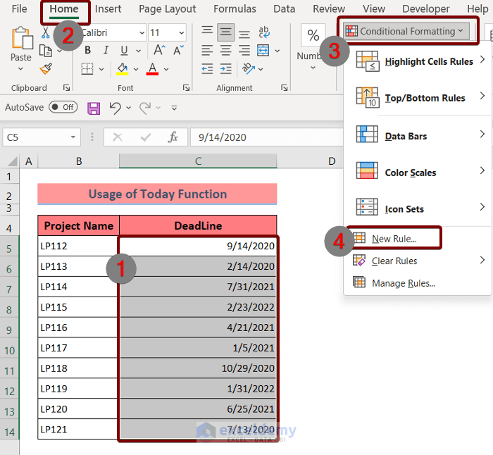
• Select the range of cells where you want to apply the conditional formatting.
• Go to Home, Conditional Formatting, and New Rule.

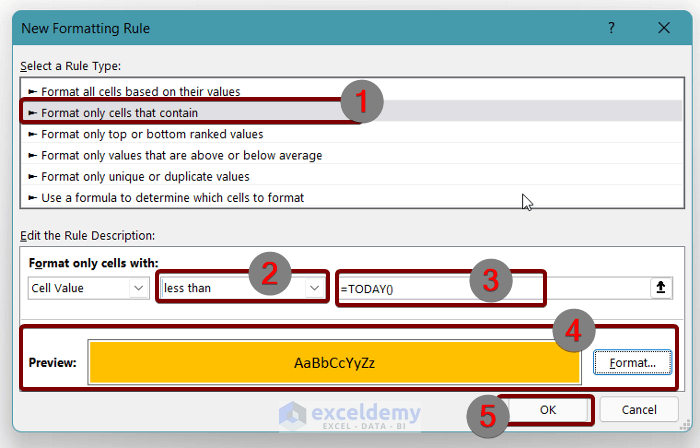
• A New Formatting Rule dialog box will pop up.
• From the dialog box, select Format only cells that contain.
• Select less than under Format only cells with field.
• In the box, insert the function

• Choose the format color using the Format option and selecting fill and text colors. We left it as orange fill.
• Hit OK.

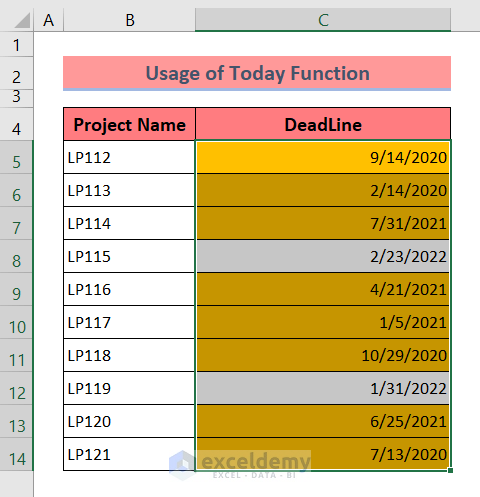
• You will get all the cells highlighted with orange color.

Read more: Excel Conditional Formatting Based on Date

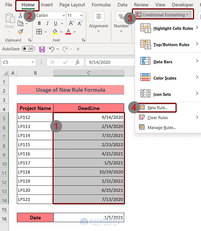
Method 3 – Use New Rule to Apply Conditional Formatting to the Overdue Dates in Excel

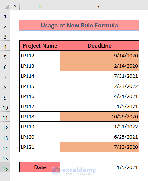
For example, we want to highlight those dates that differ more than 10 days from another inserted date which is 1/5/2021.

Steps:

• Select the range of cells where you want to apply the conditional formatting.
• Go to Home, click on Conditional Formatting, and select New Rule.

• A New Formatting Rule dialog box will appear.
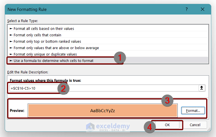
• Select Use a formula to determine which cells to format.
• Insert the following formula in the Format values where this formula is true box:

• Choose a formatting color using the Format command.
• Hit the OK button.

When you are done with all of these, you will see your intended cells are highlighted with the color that you’ve chosen using the Format command as in the picture below:

Read more: Excel Conditional Formatting for Dates within 30 Days

Things to Remember

Always select the cells before applying the Conditional Formatting command.

Press CTRL + Z to undo the Conditional Formatting command.

Download the Practice Workbook

You are recommended to download the Excel file and practice along with it.

Related Articles

• Highlighting Row with Conditional Formatting Based on Date in Excel
• Conditional Formatting Based on Date in Another Cell in Excel
  
• How to Change Cell Color Based on Date Using Excel Formula
  
• How to Apply Conditional Formatting to Each Row Individually
• How to Apply Conditional Formatting to Multiple Rows
• How to Highlight Row Using Conditional Formatting
• Conditional Formatting on Multiple Rows Independently in Excel
• How to Change Row Color Based on Text Value in Cell in Excel

<< Go Back to Conditional Formatting Based on Date | Conditional Formatting | Learn Excel