How to Apply Conditional Formatting to Each Row Individually

Conditional Formatting is a versatile feature embedded in Excel, that comes up with a lot of flexibility in terms of highlighting cells. You can apply conditional formatting to a single cell or a row as well as multiple cells or rows. It also allows you to undo your applied conditional formatting to certain cells or from the entire spreadsheet. In this article, you will receive 3 easy ways on how to apply conditional formatting to each row in Excel individually.

Here, we have used Conditional Formatting to highlight all the rows, having a quantity of more than 25. Read through the rest of the part to learn more along with some other methods in detail.

Download the Practice Workbook

You are recommended to download the Excel file and practice along with it.

3 Easy Ways to Apply Conditional Formatting to Each Row Individually

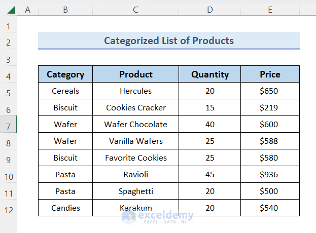
In this article, we have used a sample product price list as a dataset to demonstrate all the methods. So, let’s have a sneak peek at the dataset:

So, without having any further discussion just dive straight into all the methods one by one.

1. Using New Rule to Apply Conditional Formatting to Each Row

The new rule command allows you to create user-defined conditions based on which it can format or highlight cells. In our demo dataset, you will see a product price list having a column called Quantity. Based on the values of this column, we are going to highlight all the rows, having a quantity of more than 25. So without more delay, let’s get straight on the steps right now.

Steps:

• First of all, select the entire data table.
• Then go to Home ▶ Conditional formatting ▶ New Rule.

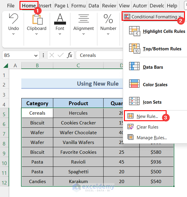
• After hitting the New Rule command, a dialog box called New Formatting Rule will appear.
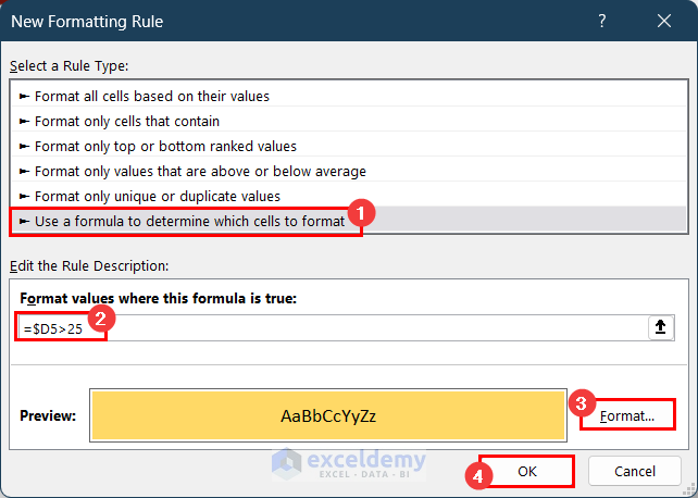
• Select Use a formula to determine which cells to format.
• Then insert the formula:

• After that pickup a color using the Format option.
• Finally hit the OK command.

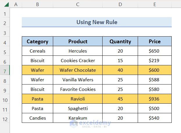
• When you are done with all the steps mentioned above, you will see two rows have been highlighted as in the image below:

Read more: How to Highlight Row Using Conditional Formatting

2. Applying Conditional Formatting to Each Row with Highlight Cells Rules

Now you have to highlight all the cells in the column Quantity, having a quantity of more than 30. To implement this, we have used the Highlight Cells Rules command here. So, without having any further discussion, let’s dive straight into the steps.

Steps:

• First of all, select the entire column of your dataset.
• Then go to Home ▶ Conditional Formatting ▶ Highlight Cells Rules.
• After approaching so far, you will have so many more options than you can utilize to format or highlight your data in your data table. But we will choose the Greater Than command among all the other options. Because we want to highlight only those values having a quantity of more than 30.

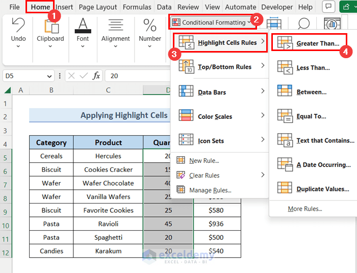
• After selecting the Greater Than command, the Greater Than dialog box will appear.
• Now, insert 30 within the insertion box.
• Then hit the OK command.

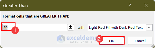
• When you are done with all the steps mentioned above, you will see the end result as in the image below:

Read more: How to Apply Conditional Formatting to Multiple Rows

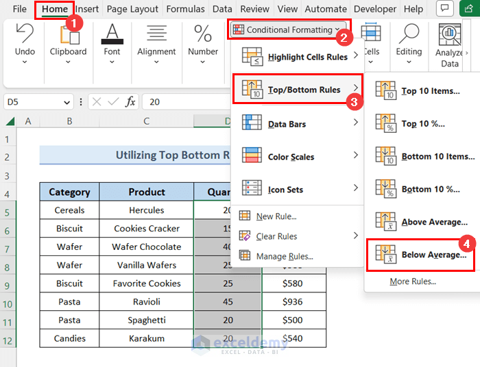
3. Utilizing Top/Bottom Rules to Apply Conditional Formatting to Each Row

Another way to apply conditional formatting to each row individually is to use the Top/Bottom Rules command. Using this command, now you have to highlight all the cells having a quantity below the average within the Quantity column. To make this thing come into action, all you need to do is follow the steps.

Steps:

• Select the entire column, Quantity.
• Then go to Home ▶ Conditional Formatting ▶ Top/Bottom Rules.
• After approaching this, we will see a bunch of options appear. Among the options, we want to pick up the Below Average command.

• After choosing the Below Average command, a dialog box named Below Average will appear. All you need to do is just hit the OK command within the pop-up dialog box.

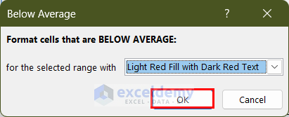
• When you are done with all the steps mentioned above, you will see the end result as illustrated in the image below:

Read more: Conditional Formatting on Multiple Rows Independently in Excel

How to Clear Rules from Each Row

After applying conditional formatting, you will feel the necessity of removing the applied formatting from a specific cell. If so, then we recommend you follow the steps below to learn to clear rules from your applied cells.

Steps:

• First of all, select the range of the cells, where you have already applied the conditional formatting.
• After the go-to Home ▶ Conditional Formatting ▶ Clear Rules ▶ Clear Rules from Selected Cells.

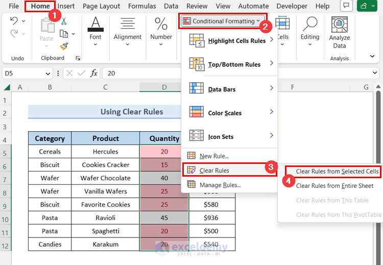
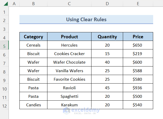
• After hitting the Clear Rules command from selected cells, you will see all of your applied cell formattings have been removed at once.

Things to Remember

📌 Always select the cells before applying the Conditional Formatting command.

📌 Press CTRL + Z to undo the Conditional Formatting command.

Conclusion

To sum up, we have provided 3 tips to apply conditional formatting to each row individually in Excel. We recommend you to download the practice workbook attached along with this article and practice all the methods with that. And don’t hesitate to ask any questions in the comment section below. We will try to respond to all the relevant queries asap. And please visit our website Exceldemy to explore more.

Further Readings

• How to Change a Row Color Based on a Text Value in a Cell in Excel
• Highlight Highest Value in Excel (3 Quick Ways)
• How to Use Conditional Formatting in Excel [Ultimate Guide]
• Excel Alternating Row Color with Conditional Formatting [Video]