Here’s the overview of the functions we’ll use today and how they highlight cells or rows based on dates or ranges.
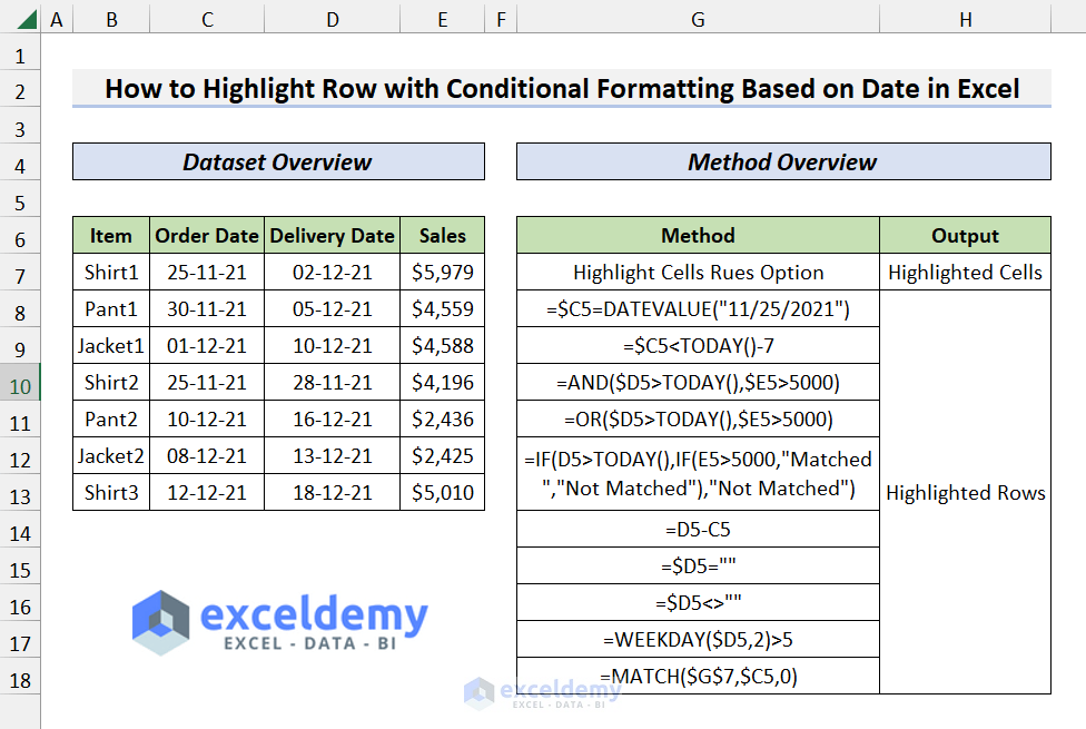
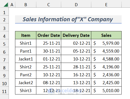
We have a data table with the Sales value, Order Date, and Delivery Date for different items. The date format is dd/mm/yyyy.
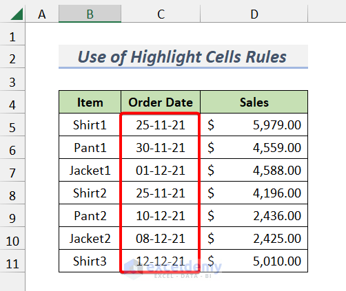
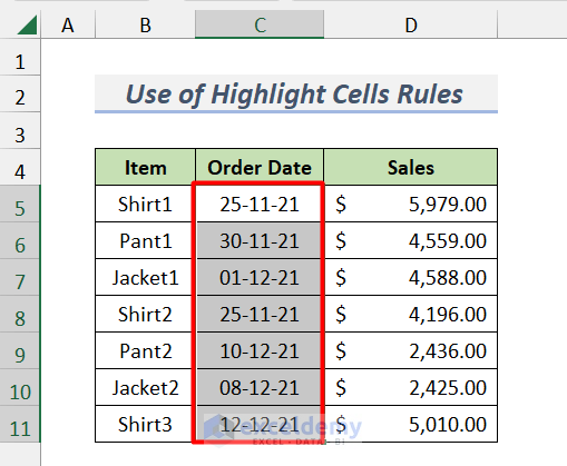
Method 1 – Using Highlight Cells Rules Option to Conditionally Format Rows Based on Date in Excel
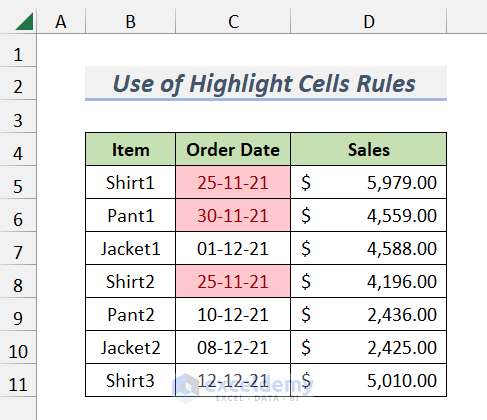
We’ll highlight cells with dates in the previous month.
Steps:
- Select the data range on which you want to apply the Conditional Formatting. We selected C5:C11.
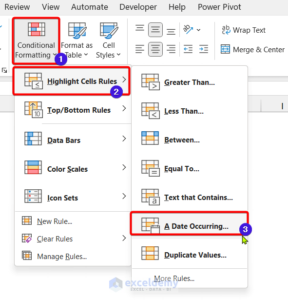
- Go to the Home tab.
- Click on the Conditional Formatting dropdown.
- Choose Highlight Cells Rules and select the A Date Occurring option.
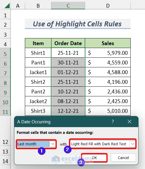
- A Date Occurring Wizard will open.
- Select the Last Month option from the dropdown on the left and use any formatting you like.
- The last month’s Order Dates will be highlighted as below.
Read more: Excel Conditional Formatting Based on Date
Method 2 – Highlighting Specific Dates with Excel Conditional Formatting
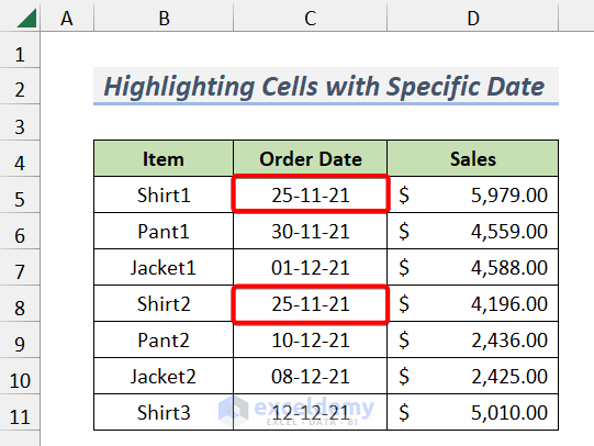
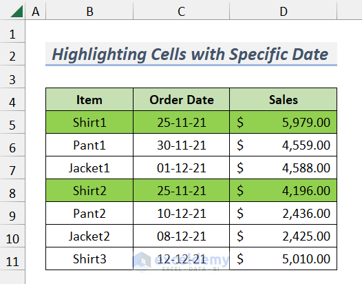
Let’s say you want to highlight the rows that have a specific date. We’ll use the date constant as 25-11-2021.
Steps:
- Select the data range on which you want to apply the Conditional Formatting.
- Go to the Home tab and choose Conditional Formatting.
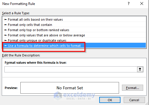
- Select New Rule.

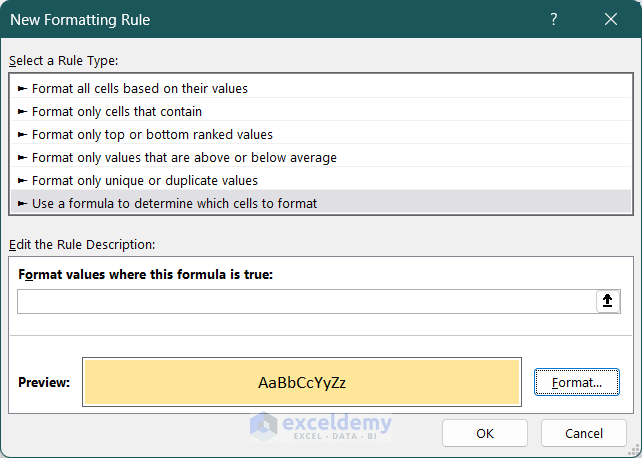
- The New Formatting Rule Wizard will appear.
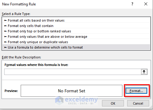
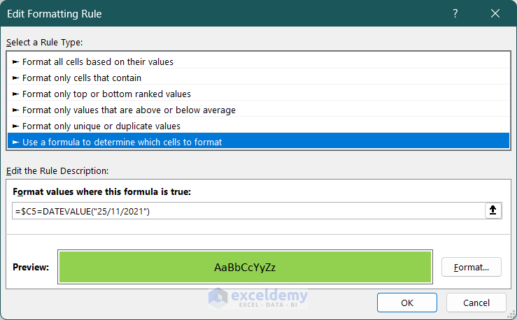
- Select the Use a formula to determine which cells to format option.
- Click on the Format button.
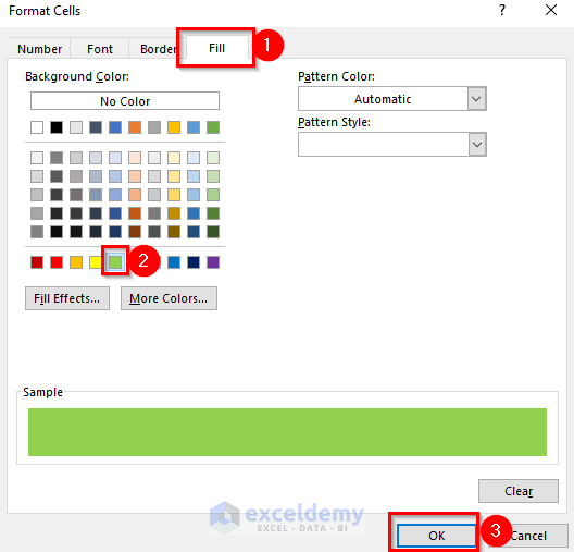
- Under Fill, select a background color.
- Click on OK.
- The Preview will be shown below.
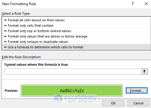
- Use the following formula in the Format values where this formula is true: box.
=$C5=DATEVALUE("25/11/2021")When the cells of Column C are Equal to the date 11/25/2021, then the Conditional Formatting will appear in those rows. The DATEVALUE function will convert the text date into a value.
- Press OK.
- You will get the rows with the specific date 25/11/2021 highlighted.
Read more: Conditional Formatting Based on Date in Another Cell in Excel
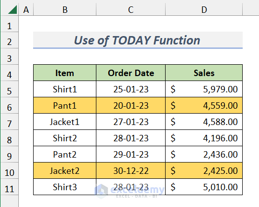
Method 3 – Using the TODAY Function to Highlight Dates by Excel Conditional Formatting
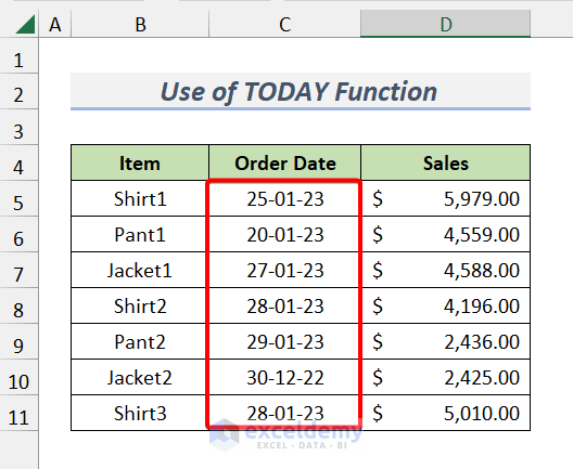
Suppose you want to highlight the dates before the past seven days in the Order Date column.
Steps:
- Open the New Formatting Rule dialogue box from the Conditional Formatting option on the Home tab ribbon.
- Use the following formula in the Format values where this formula is true: box.
=$C5<TODAY()-7- Press OK.
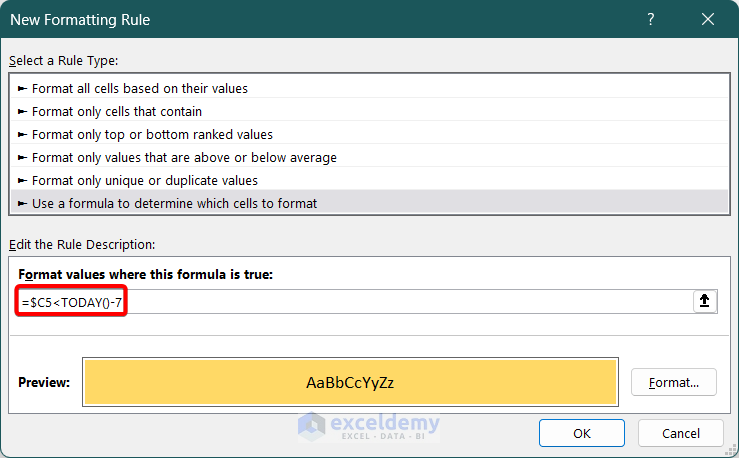
- You will get the rows highlighted.
Note: If you want to find values older than 1 year, your formula will be:
=$C5<TODAY()-365
Read more: Apply Conditional Formatting for Dates Older Than Today in Excel
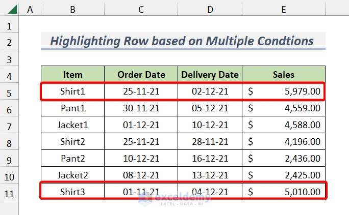
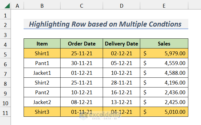
Method 4 – Highlighting Rows Based on Date for Multiple Conditions Using the AND Function
Let’s to highlight the rows which have delivery dates before 05/12/2021 and the sales value greater than $5,000.
Steps:
- Open the New Formatting Rule dialogue box from the Conditional Formatting option on the Home tab ribbon.
- You will get the following New Formatting Rule dialog box.
- Use the following formula in the Format values where this formula is true: box.
=AND($D5<DATE(2021,12,5),$E5>5000)- Press OK.
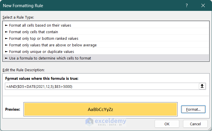
- This will highlight the applicable rows.
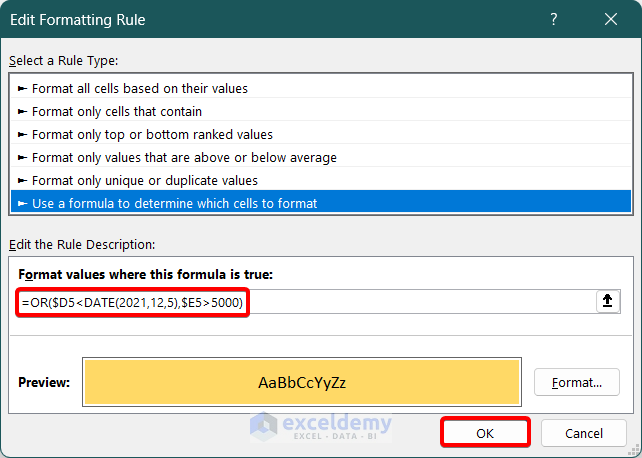
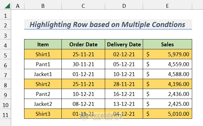
Method 5 – Using the OR Function to Highlight Rows Based on Date for Multiple Conditions
Let’s highlight the rows that have delivery dates before 05/12/2021 or a sales value greater than $5,000.
Steps:
- Open the New Formatting Rule dialogue box from the Conditional Formatting option on the Home tab ribbon.
- Use the following formula in the Format values where this formula is true: box.
=OR($D5<DATE(2021,12,5),$E5>5000)- Press OK.
- Here are the results for our sample.
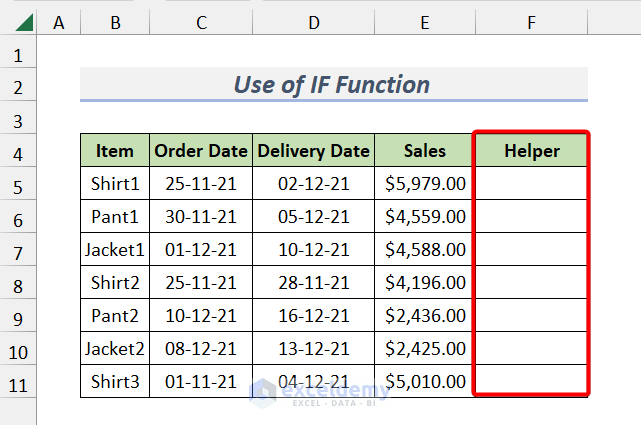
Method 6 – Applying Excel Conditional Formatting Based on Date for Multiple Conditions Using the IF Function
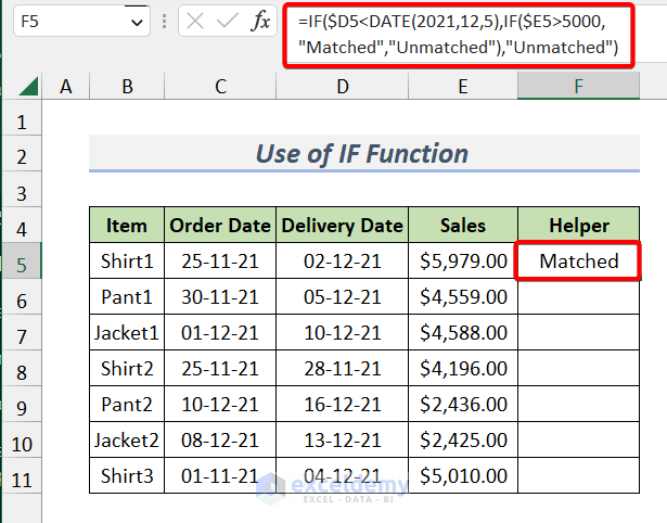
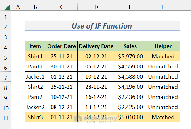
We have added a column named Helper. We want to highlight the rows which have delivery dates before 05/12/2021 and a sales value greater than $5,000.
Steps:
- Select the output Cell F5.
- Use the following formula and press Enter.
=IF($D5<DATE(2021,12,5),IF($E5>5000,"Matched","Unmatched"),"Unmatched")- IF will return “Matched” if both the conditions are met.
- Drag down the Fill Handle tool.

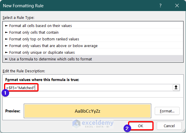
- Open the New Formatting Rule dialog box.
- Use the following formula in the Format values where this formula is true: box.
=$F5="Matched"- Press OK.
- Here are the results.
Read more: Excel Conditional Formatting Formula with IF
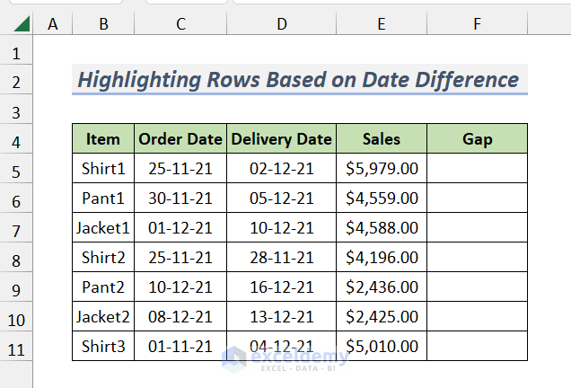
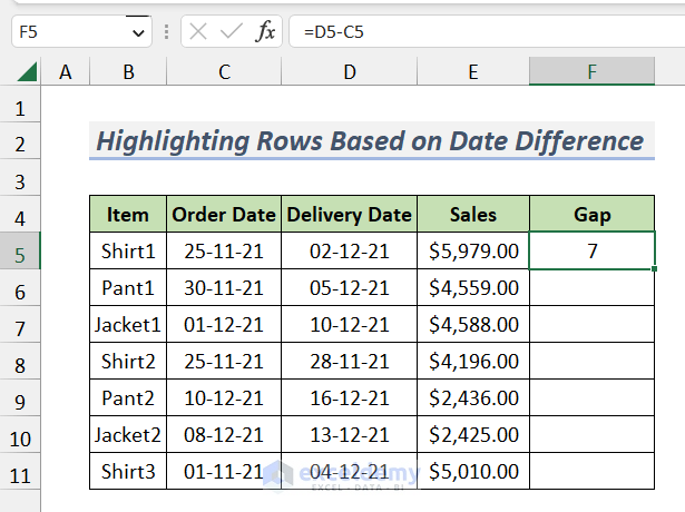
Method 7 – Conditional Formatting Based on Gaps Between Dates
Suppose you want to highlight the rows with a difference between the Delivery Date and Order Date less than 6 days (for highlighting the fast delivery rows). We have added a column named Gap.
Steps:
- Select the output Cell F5.
- Use the following formula and press Enter.
=D5-C5- This will return the gaps between the two dates (Delivery Date and Order Date).
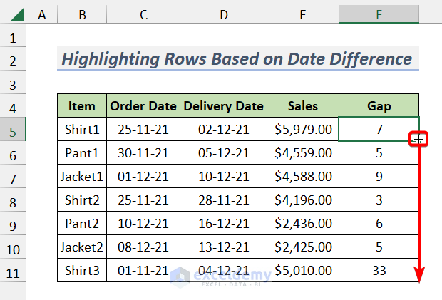
- Drag down the Fill Handle tool.
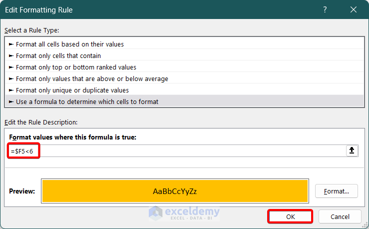
- Open the New Formatting Rule dialog box.
- Use the following formula in the Format values where this formula is true: box.
=$F5<6- Press OK.
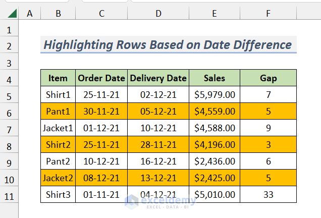
- Here are the results.
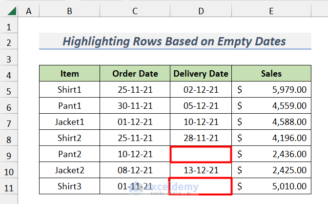
Method 8 – Highlighting Rows Based on Empty Dates with Excel Conditional Formatting
Let’s highlight the rows where the Delivery Date is empty. We’ve removed a few dates from the dataset.
Steps:
- Open the New Formatting Rule dialog box.
- Use the following formula in the Format values where this formula is true: box.
=$D5=""- Press OK.
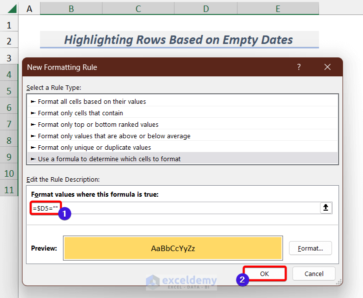
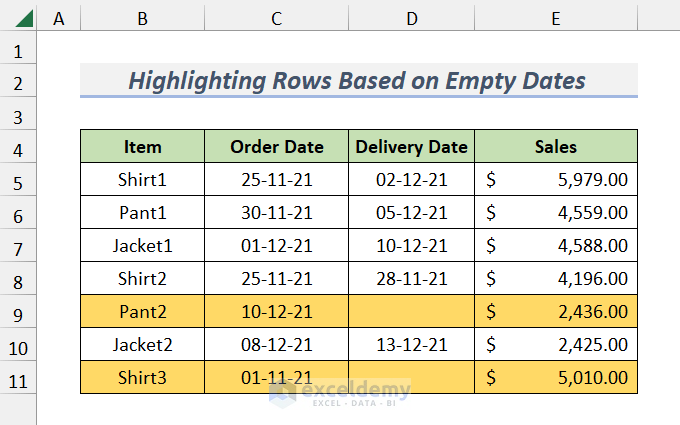
- Here are the results.
Read more: Conditional Formatting for Blank Cells in Excel
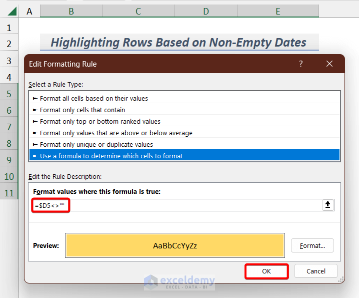
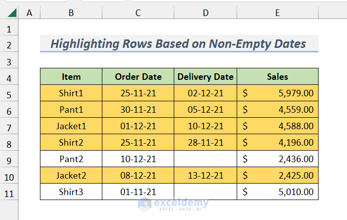
Method 9 – Applying Conditional Formatting to Rows Based on Non-Empty Dates
Steps:
- Select cells B5:E11 and follow the steps of Method 2 to open the New Formatting Rule dialog box.
- Use the following formula in the Format values where this formula is true: box.
=$D5<>""- Press OK.
- Here are the results.
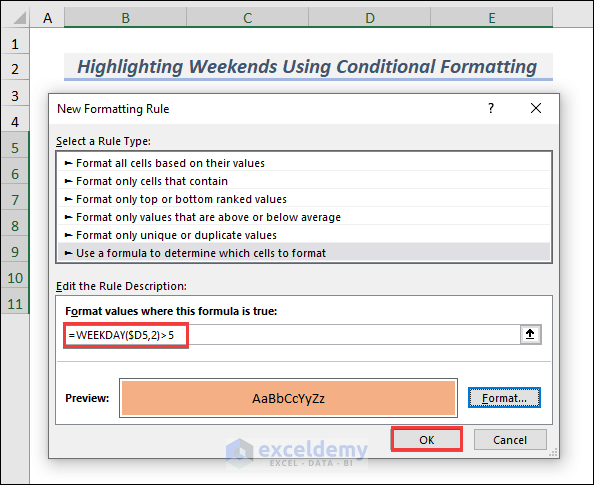
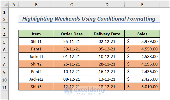
Method 10 – Highlighting Weekends Using Excel Conditional Formatting and the WEEKDAY Function
Let’s highlight rows that have Saturdays and Sundays in the Delivery Date.
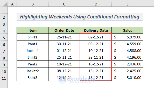
Steps:
- Select cells B5:E11 and follow the steps of Method 2 to open the New Formatting Rule dialog box.
- Use the following formula in the Format values where this formula is true: box.
=WEEKDAY($D5,2)>5When the values will be 6 and 7, then the Conditional Formatting will appear in the corresponding rows.
- Press OK.
- You will get the rows highlighted for weekends.
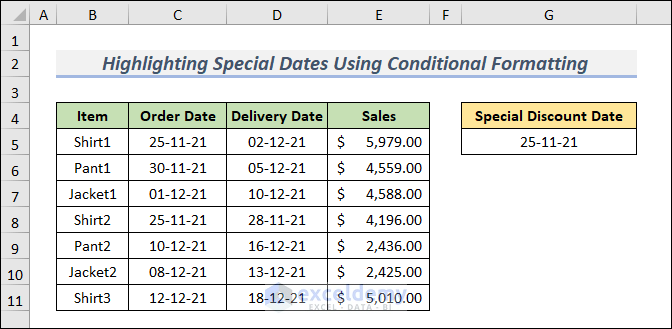
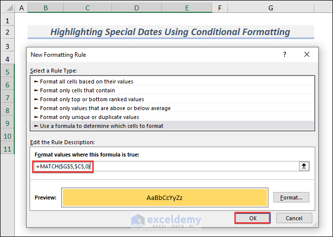
Method 11 – Applying Excel Conditional Formatting to Highlight Special Dates
We have created a new cell that will be used to hold the search value for the Order Date.
Steps:
- Select cells B5:E11 and follow the steps of Method 2 to open the New Formatting Rule dialog box.
- Use the following formula in the Format values where this formula is true: box.
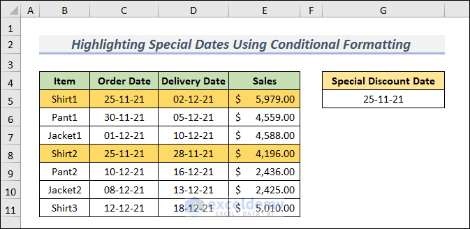
=MATCH($G$5,$C5,0)- Press OK.
- Here are the results.
Download the Practice Workbook
Further Readings
- How to Change Cell Color Based on Date Using Excel Formula
- Apply Conditional Formatting to Overdue Dates in Excel
- Excel Conditional Formatting for Dates within 30 Days
- How to Apply Conditional Formatting to Each Row Individually
- How to Apply Conditional Formatting to Multiple Rows
- Conditional Formatting on Multiple Rows Independently in Excel
- How to Change Row Color Based on Text Value in Cell in Excel
<< Go Back to Conditional Formatting Based on Date | Conditional Formatting | Learn Excel
Get FREE Advanced Excel Exercises with Solutions!
