Conditional Formatting Based on Date in Another Cell in Excel

Conditional formatting is a useful Excel feature that allows you to show data in a more organized fashion. It is extremely helpful for displaying date information as well. In this article, I have provided 3 ways to apply conditional formatting to the cells based on the date in another cell in Excel. In this section, you’ll explore how to apply the conditional formatting feature, considering either the date in a specific cell or the cells between two dates. I’ll even show you if the date is in another column. Let’s dive into the methods.

1. Using Conditional Formatting Based on Date in Another Particular Cell

This method shows how you can apply Excel conditional formatting to selected cells based on a date in a particular cell.

excel conditional formatting based on date in a particular cell

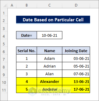
Here, I have formatted the rows where the joining dates are after a specific date.

Follow these steps to apply this solution:

First, select the cells you want to apply the conditional formatting on (In my case, B7:D11).
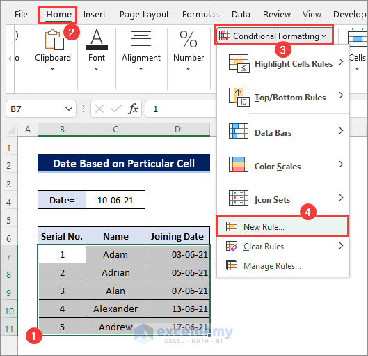
Then, go to Home >> Conditional Formatting >> New Rule as shown below.

Home >> Conditional Formatting >> New Rule

After that, a new window named New Formatting Rule should appear. Next, select Use a formula to determine which cells to format rule type.
Then, enter the condition/formula in the specified field (In my case, =$D9>$C$4) and select the Format This will open the Format Cells dialog box. Now apply the formatting as required (in this case, Font >> Font Style >> Bold and Fill >> Background Color >> Yellow) and click OK twice.

=$D9>$C$4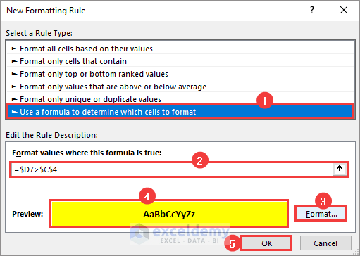

conditional formatting rule

Finally, the selected cells will be formatted according to the condition and selected format.

Explanation: The dollar sign ($) is known as the Absolute Symbol. It makes the cell references absolute and doesn’t allow any changes. You can lock a cell by selecting the cell and pressing the F4 button.

Here, $C$4 means that the C4 cell is locked for every reference. It will not change. The $D7 indicates that the column D reference is absolute, it will not change, but the rows will adjust accordingly.

So, =$D7>$C$4 this formula will output the rows where the joining dates of employees (column D) are after the specific date (Cell C4).

2. Applying Excel Conditional Formatting Between Two Dates in Another Cells

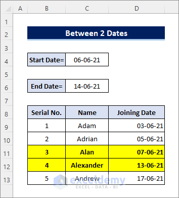
This method shows how to apply Excel conditional formatting in selected cells based on two dates in different cells.

Here, I have formatted the rows where the joining dates are between two different cell dates.

excel conditional formatting based on date between two dates

Follow these steps to apply this solution:

First, select the cells you want to apply the conditional formatting on (In my case, B9:D11).
Then, go to Home >> Conditional Formatting >> New Rule and select Use a formula to determine which cells to format rule type as earlier.
Next, enter the condition/formula in the specified field (In my case, =AND($D9>=$C$4, $D11<=$C$6)), click on Format to apply the desired formatting, and click OK.

=AND($D9>=$C$4, $D11<=$C$6)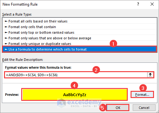

new formatting rule

Here, =AND($D9>=$C$4, $D9<=$C$6) this formula checks whether the dates in column D are greater than the C4 cell’s date and less than the C6 cell’s date. The AND function returns TRUE only when all of the conditions are met. If the date satisfies the conditions, the selected cells will be formatted according to the condition and selected format.

3. Using Conditional Formatting Tool Based on Dates in Another Column

This method shows how to apply Excel conditional formatting to selected cells based on another column.

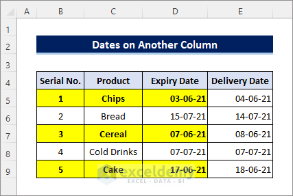
Here, I have formatted the cells and highlighted the products that were delivered after the expiration date.

excel conditional formatting based on date in another column

Follow these steps for applying this solution:

First, select the cells you want to apply the conditional formatting on (In my case, B5:D9).
Then, go to Home >> Conditional Formatting >> New Rule and select Use a formula to determine which cells to format rule type as earlier.
Next, enter the condition/formula in the specified field (In my case, =$D5<$E5) and click on Format to apply the desired formatting.

=$D5<$E5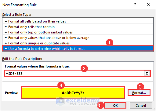

conditional formatting rule

Here, =$D5<$E5 this formula checks whether the dates in column D are less than the dates in column E. If the date satisfies the conditions, then the selected cells will be formatted according to the condition and selected format.

Using Conditional Formatting Based on Date Older Than 1 Year

This method shows how to apply Excel conditional formatting to selected cells based on dates older than 1 year.

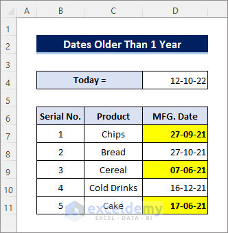
Here, I have formatted the cells and highlighted the manufacturing dates that are older than a year.

excel conditional formatting based on date older than 1 year

Follow these steps to apply this solution:

First, select the cells you want to apply the conditional formatting on (In my case, D7:D11).
Then, go to Home >> Conditional Formatting >> New Rule and select Use a formula to determine which cells to format rule type as earlier.
Next, enter the condition/formula in the specified field (In my case, =D7<TODAY()-365) and click on Format to apply the desired formatting.

=D7<TODAY()-365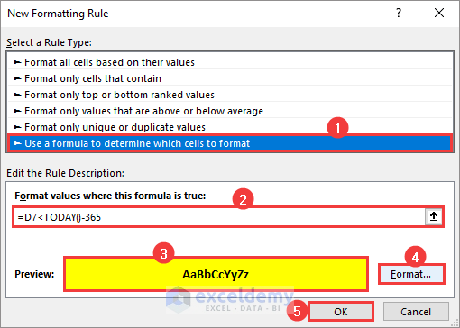

formatting rule

Here, the TODAY function outputs the current date, which is, in this case, 12-10-22. So, TODAY()-365 returns a date going back to 365 days i.e. 1 year earlier. Therefore, =D7<TODAY()-365 this formula checks whether the dates in column D are older than a year. If the date satisfies the conditions, then the selected cells will be formatted according to the condition and selected format.

Applying Conditional Formatting Based on Date Before Today

This method shows how to apply conditional formatting to selected cells based on dates before today.

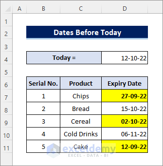
Here, I have formatted the cells and highlighted the expiry dates which were before today.

excel conditional formatting based on date before today

Follow these steps to apply this solution:

First, select the cells you want to apply the conditional formatting on (In my case, D7:D11).
Then, go to Home >> Conditional Formatting >> New Rule and select Use a formula to determine which cells to format rule type as earlier.
Next, enter the condition/formula in the specified field (In my case, =D5<TODAY()) and click on Format to apply the desired formatting.

=D5<TODAY()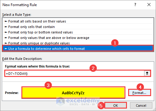

format condition

Here, =D7<TODAY() this formula checks whether the dates in column D refer to dates earlier than today. If the date satisfies the conditions, then the selected cells will be formatted according to the condition and selected format.

Things to Remember

Notice carefully when to use the Absolute, Mixed, or Relative cell references in the formulas. Using the wrong type of cell references may not return the desired result.
You must enter dates according to the system date formatting (dd/mm/yy, mm/dd/yy, etc) on your PC.

Download Practice Workbook

You can download the workbook that I used in this article from below and practice with it by yourself.

Conditional Formatting Based on Date in Another Cell.xlsx

Conclusion

In Microsoft Excel, conditional formatting is a powerful tool. I have used this feature in this article and narrowed down 3 popular ways to apply Excel conditional formatting based on a date in another cell. I hope you find the solution you were looking for. Please leave a comment if you have any suggestions or questions.