Without a doubt, Conditional Formatting is a nifty feature of Excel that allows us to highlight cells based on any criteria. So, we can, at a glance, locate the cells that satisfy the given condition. Granted this, in this article, we’ll describe 5 ways how to apply Conditional Formatting to multiple rows.
The GIF below is an overview of the article which represents the application of Conditional Formatting to multiple rows.
In the following sections, we’ll learn about the dataset and explore each method in detail and with the proper illustrations.
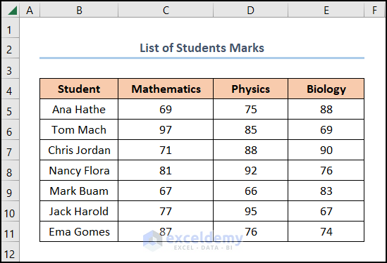
First and foremost, let’s consider the List of Students Marks dataset shown in the B4:E11 cells containing the “Student”, “Mathematics”, “Physics”, and “Biology” columns respectively. Here, we want to highlight those cells with scores greater than 79. Therefore, let’s see it in action.
Here, we have used the Microsoft Excel 365 version; you may use any other version at your convenience.
1. Highlighting Multiple Rows with Conditional Formatting
In the first place, let’s start with the simplest way to apply Conditional Formatting to multiple rows. Now allow us to demonstrate the process in the steps below.
📌 Steps:
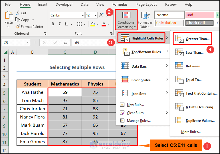
- First of all, select all the cells, in this case, C5:E11 >> go to Conditional Formatting >> Highlight Cell Rules >> select the Greater Than option.
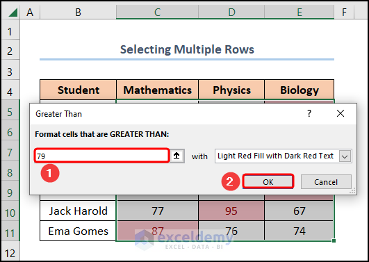
Now, a Greater Than window appears.
- Next, in the Format cells that are GREATER THAN box, enter 79 >> click on OK.
Ta-dah! That is how simple it is to apply Conditional Formatting to multiple rows.

Read More: How to Apply Conditional Formatting to Each Row Individually
2. Applying Conditional Formatting to Multiple Rows with Paste Special Feature
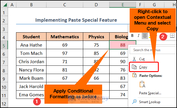
Besides, we can use the Paste Special option to copy-paste the Conditional Formatting if one of the cells already has been formatted. Suppose, cell E5 is highlighted based on the condition that its value is greater than 79 and now we want to apply the same formatting in all other rows.
📌 Steps:
- Initially, follow the steps shown previously to apply Conditional Formatting to the E5 cell >> Right-click to open the Contextual menu >> click on Copy.
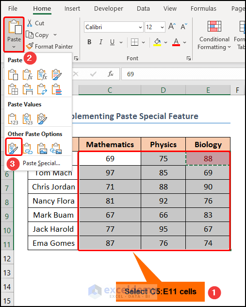
- Then, select the C5:E11 cells >> press the Paste drop-down >> choose the Paste with Formatting option.
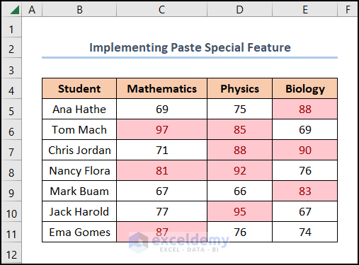
Finally, the results should look like the image given below.
Read More: How to Highlight Row Using Conditional Formatting
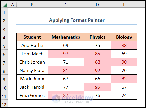
3. Applying Conditional Formatting to Multiple Rows with Excel Format Painter
Alternatively, Format Painter is another amazing feature of Excel by which we can easily apply the format of one cell to other cells. Therefore, just follow along.
📌 Steps:
- At the very beginning, apply Conditional Formatting to the E5 cell by following the previous steps >> observe the live demonstration as shown in the animated GIF.
Eventually, the final output should look like the picture shown below.
Read More: Conditional Formatting on Multiple Rows Independently in Excel
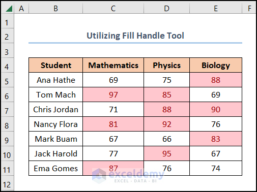
4. Using Fill Handle Tool to Apply Conditional Formatting to Multiple Rows
For one thing, we can also implement the Fill Handle tool to apply conditional formatting to multiple rows by dragging the formatted cells.
📌 Steps:
- In this scenario, Conditional Formatting is already applied to the C5 cell as shown prior >> Observe the GIF to follow the steps in real-time.
Boom! The final output should resemble the figure shown below.
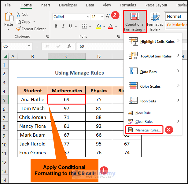
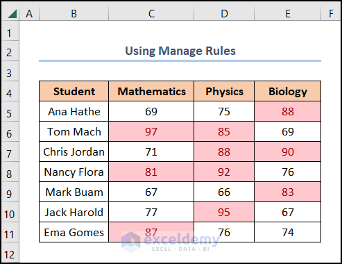
5. Using Manage Rules to Apply Excel Conditional Formatting to Multiple Rows
Last but not least, the Manage Rules feature within the Conditional Formatting drop-down can also be used to format multiple rows. Now, allow us to demonstrate the process in the steps below.
📌 Steps:
- First, select the C5 cell that has Conditional Formatting >> move to Conditional Formatting >> choose the Manage Rules option.
Not long after, the Conditional Formatting Rules Manager wizard pops out.
- At this point, in the Applies to box insert the C5:E11 cell range >> click Apply >> hit OK.

Consequently, your final output should appear in the screenshot given below.
Download Practice Workbook
Conclusion
To sum up, we hope this article helps you understand how to apply Conditional Formatting to multiple rows. Now, if you have any queries, please leave a comment below.
Conditional Formatting Rows in Excel: Knowledge Hub
- Apply Conditional Formatting to Each Row Individually
- Highlight Row Using Conditional Formatting
- Conditional Formatting on Multiple Rows Independently
- Change Row Color Based on Text Value in Cell
<< Go Back to Conditional Formatting | Learn Excel
Get FREE Advanced Excel Exercises with Solutions!

Very good, however, if I want to copy conditional formatting from cell J3 to J34 but also the Cell Value move in line with the row.
Example.
I copy conditional formatting from cell J3 to J4 but the new J4 conditional format still looks at the data in D3 and not D4.
This repeats over multiple cells, if I copy CF from J3 and Format Painter from J4 to J34 every cell from J4 to J34 looks at D3 for the value rather than column D on the same row.
Only way around is to do each cell individual or go into CF manager and update each one.
Does anyone has a solution, something like an option to change in Excel 🙂
If you look at our method 5, we have tried to apply conditional formatting based on a certain condition. The value was fixed all along the applied range.
HELLO
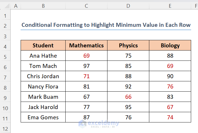
I NEED TO APPLY A CONDITIONAL FORMATING (THE MINIMUM MALUE) IN ROW TO MULTIPLE ROW ROW BY ROW
Hi JAD,
I hope you are doing well. Thank you very much for reading our articles.
You want to apply conditional formatting to the minimum value in each row across multiple rows. For that, you need to use a formula in the conditional formatting. Follow the instructions given below:
=C5=MIN($C5:$E5)You can see minimum values of each row have been highlighted.
Regards,
Alok Paul
ExcelDemy Team