How to Change Row Color Based on Text Value in Cell in Excel

Written by Asikul Himel

Last updated: Jul 4, 2024

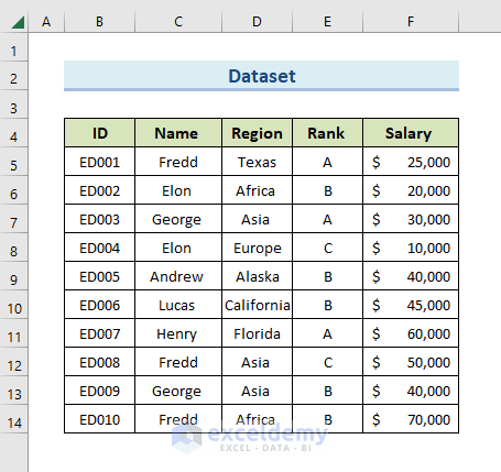
We’ll use the following simple dataset to showcase how to change row colors based on text values inside cells.

Preview of change a row color based on a text value in a cell in excel

Change the Row Color Based on the Text Value in a Cell in Excel: 3 Suitable Ways

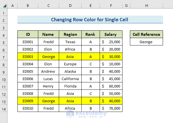
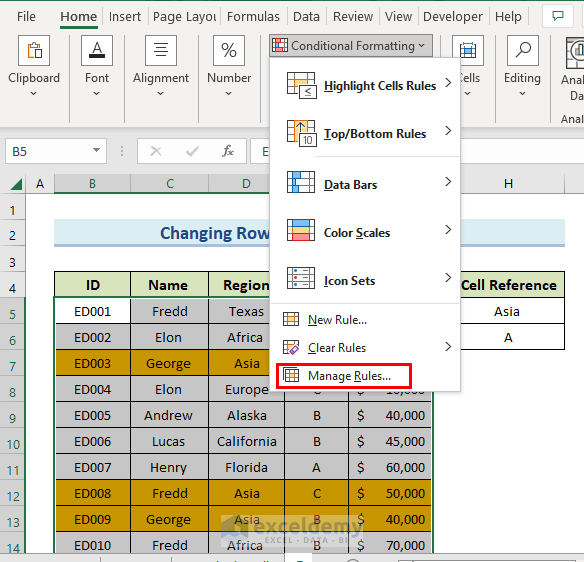
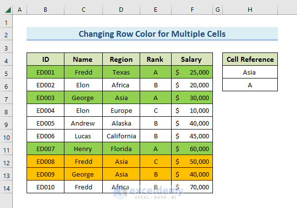
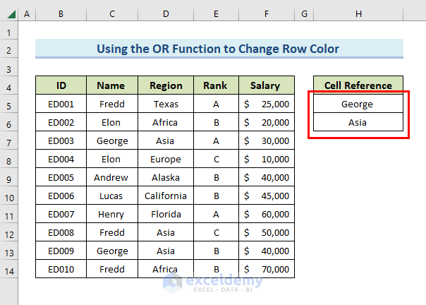
Consider the following dataset with the information for ID, Name, Region, Rank, and Salary of some Sales Representatives. We’ll change some row colors based on the names, regions, or salaries.

dataset

Method 1 – Changing the Row Color Based on Text Value

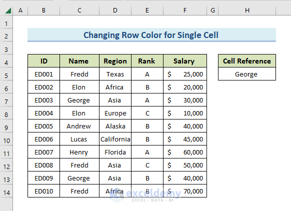
Case 1.1 – For Single Cell Criteria

We have to color the rows that have George’s name in them. We put that value in a separate cell H5.

Steps:

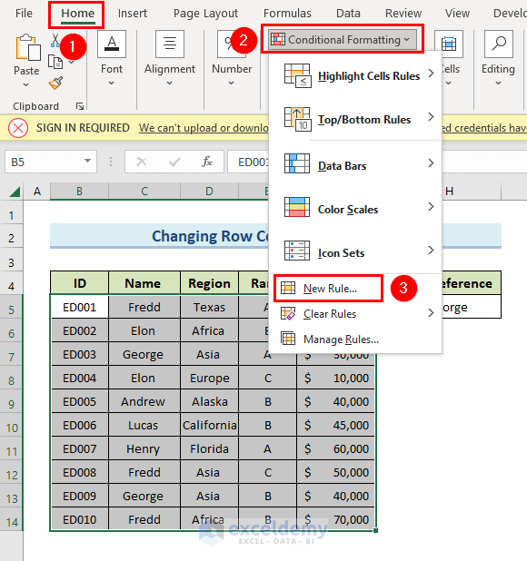
Select the entire dataset.
In your Home tab, go to Conditional Formatting in Style Group.
Click on New Rule.

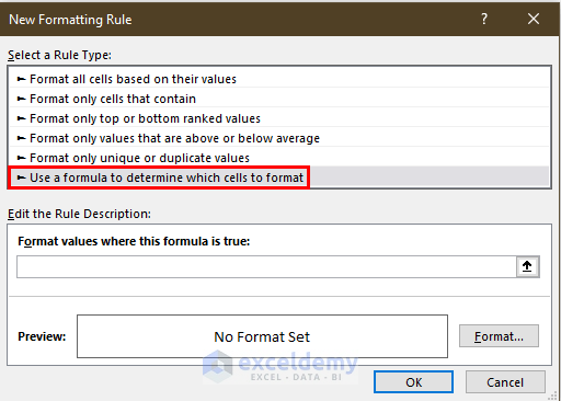
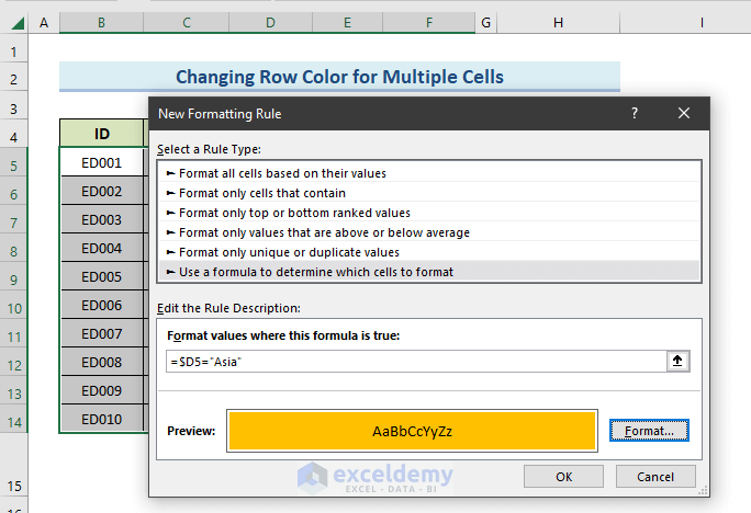
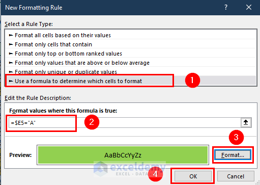
The New Formatting Rule dialog box opens. Select Use a Formula to determine which Cells to format to continue.

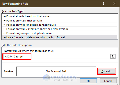
In the formula section, insert this formula.

=$C5="George"

Click on the Format option.

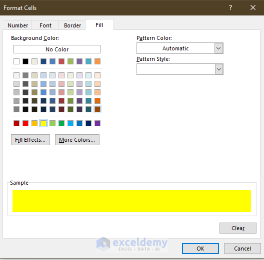
We have chosen the color of the text as Automatic. Go to the Fill tab and pick a background color. In this case, we chose the Yellow color.
Click OK.

Click OK.

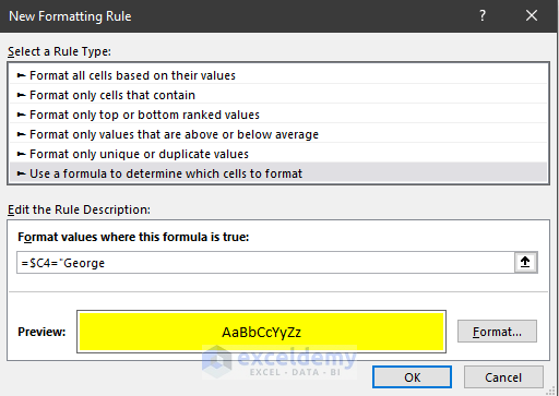
Our row colors are changed based on a text value in a cell.

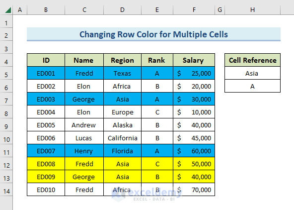
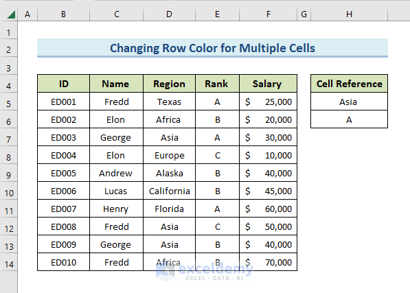
Case 1.2 – For Multiple Cell Criteria

Consider a case where you have to color the rows that have Asia and rank A in them.

Steps:

Go to the New Formatting Rule dialog box following the steps of Method 1.1.
Select Use a formula to determine which cells to format.
Insert the following formula:

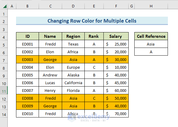
=$D5="Asia"

Select the color format for your matched cells.
Click OK.

The conditional formatting feature successfully colors the rows.

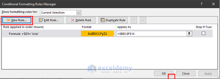
Go to Conditional Formatting and select Manage Rules.

The Conditional Formatting Rules Manager window appears. Click New Rule to add another one.

Set the following formula for the second condition:

=$E5="A"

Set the format.

Click OK to change the row color based on multiple conditions.

Press OK in the next window.

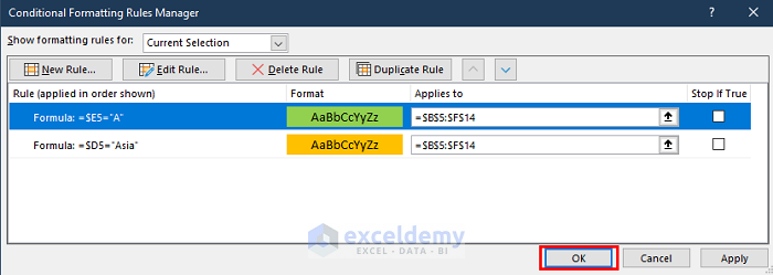
Here are the results.

Read More: How to Change Cell Color Based on Date Using Excel Formula

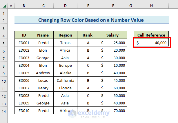
Method 2 – Altering Row Color Based on a Number Value in Excel

We have to change the row colors for employees with a salary of less than 40,000$.

Steps:

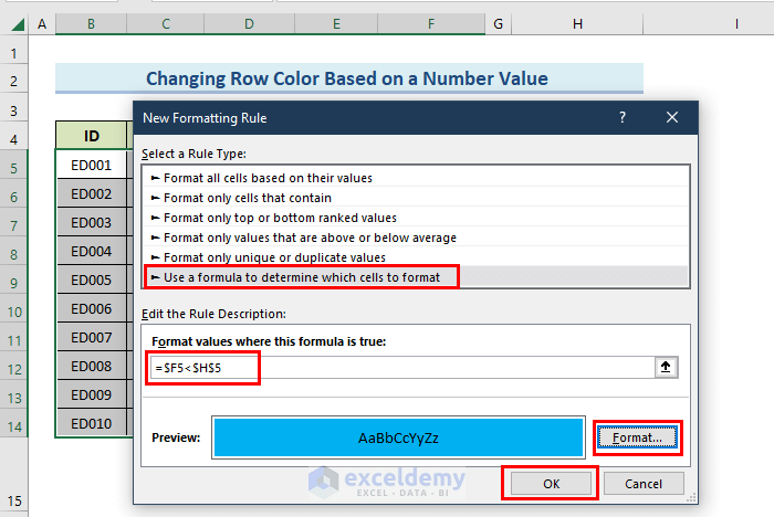
Go to New Formatting Rule (see Method 1.1).
Insert the following formula:

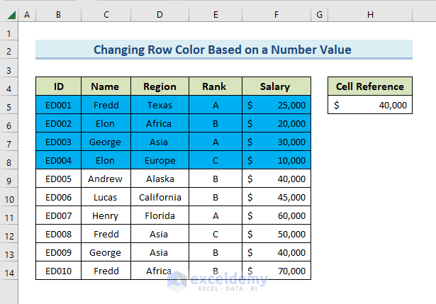
=$F5<$H$5

Specify the formatting and click OK to continue.

Here are the results.

Read More: How to Highlight Row Using Conditional Formatting

Method 3 – Applying a Formula to Change the Row Color Based on a Text Value

Case 3.1 – Using theOR Function

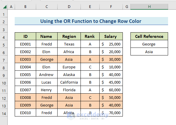
We want to color rows that contain George or Asia. Insert those texts into your reference table.

Steps:

Insert the following formula in the New Formatting Rule window.

=OR($C5="George",$D5="Asia")

Select a formatting style according to your preferences.

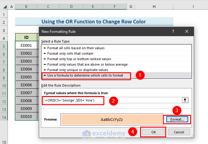
Click OK.

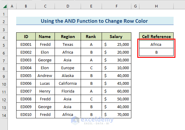
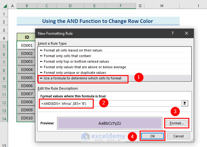
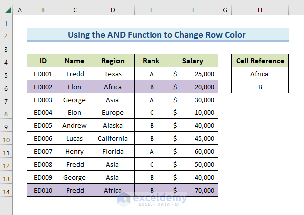
Case 3.2 – Inserting AND Function

We will change row colors that have both Africa for the region and B rank in them.

Steps:

Go to the New Formatting Rule window and apply the following formula:

=AND($D4="Africa",$E4="B")

Set the formatting style and click OK to format the cells.

Here’s the result.

Read More: Conditional Formatting on Multiple Rows Independently in Excel

Things to Remember

You can clear the rules once the formatting is applied

Use the Absolute Cell references ($) for column references to ensure that the conditional formatting is applied on the row.

Download the Practice Workbook

Changing Row Color Based on Text Value in Cell.xlsx

Similar Articles to Explore

<< Go Back to Conditional Formatting Rows | Conditional Formatting | Learn Excel

Get FREE Advanced Excel Exercises with Solutions!

SaveSavedRemoved 0

Tags: Conditional Formatting Rows in Excel

Asikul Himel

Asikul Islam Himel, holding a BSc in Naval Architecture and Marine Engineering from Bangladesh University of Engineering and Technology, has contributed over two years to the ExcelDemy project. Starting as an Excel & VBA Content Developer, now he manages projects at You Have Got This Math Project. He wrote 60+ articles for ExcelDemy, reviewed 500+, and focused on quality maintenance. Currently, his responsibilities include project management and team leadership. Himel's interests encompass data analysis, leadership, WordPress applications, and... Read Full Bio

4 Comments

Reply
Iona May 15, 2024 at 3:44 AM

I currently have a formula on my dates to turn red once 7 days overdue. However, if I want to turn the dates back to black once the cell has been filled with green paint, how can I code this in?

Thanks
- Reply
  Lutfor Rahman Shimanto May 15, 2024 at 12:52 PM
  Dear Iona
  
  Thanks for visiting our blog and sharing your requirements! I have reviewed your goal and created an Excel VBA Event procedure (assuming your dates are in column A).
  
  Excel VBA Event Procedure:
```
Private Sub Worksheet_Change(ByVal Target As Range)

    Dim cell As Range

    If Not Intersect(Target, Range("A:A")) Is Nothing Then
        For Each cell In Target
            If cell.Value < (Date - 7) And cell.Interior.Color <> RGB(0, 255, 0) Then
                cell.Font.Color = RGB(255, 0, 0)
            ElseIf cell.Interior.Color = RGB(0, 255, 0) Then
                cell.Font.Color = RGB(0, 0, 0)
            End If
        Next cell
    End If
    
End Sub
```
  Right-click on the sheet name tab, paste the given code into the sheet module and save it. Hopefully, the idea will fulfil your goal; good luck.
  
  Regards
  Lutfor Rahman Shimanto
  Excel & VBA Developer
  ExcelDemy
Reply
Sandy May 17, 2024 at 9:00 PM

Trying to conditionally format a cell to shade when a formula result from another column [@DATE] equals either Saturday or Sunday and it’s the formula in the first column that is blocking that conditional formatting. Can you write conditional formatting based on a cell that is using a formula itself?
- Reply
  Shamima Sultana May 19, 2024 at 12:28 PM
  
  Hello Sandy,
  
  You can use this formula:
  =OR(WEEKDAY([@DATE], 2) = 6, WEEKDAY([@DATE], 2) = 7)
  This checks if the [@DATE] column value is a Saturday (6) or Sunday (7).
  
  Regards
  ExcelDemy

Leave a reply Cancel reply

Submit Excel Problem