Conditional Formatting on Multiple Rows Independently in Excel

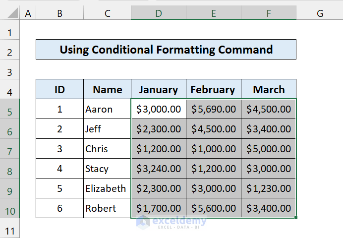
Method 1 – Use of the Conditional Formatting Command for Multiple Rows

Steps

① Select the range of cells D5:F10.

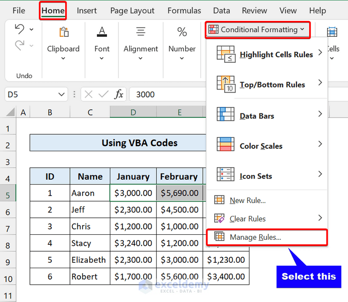
② From the Home tab, go to Conditional Formatting > Manage Rules.

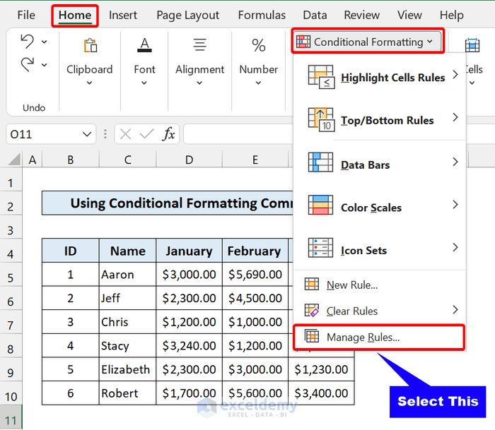
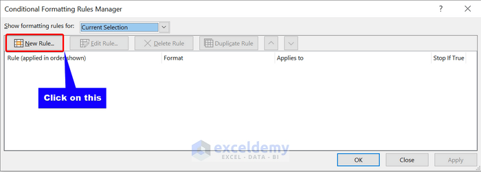
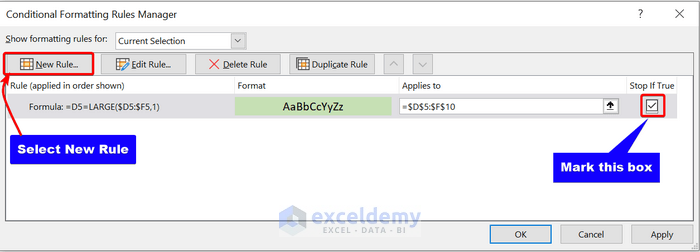
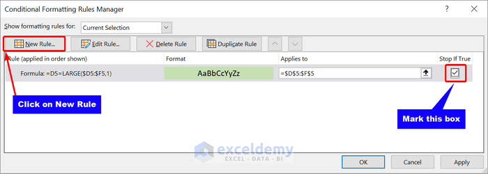
③ The Conditional Formatting Rules Manager dialog box will pop up. Click on New Rule.

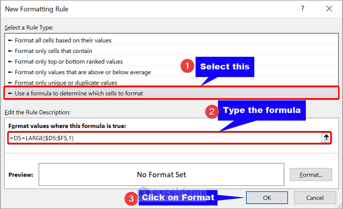
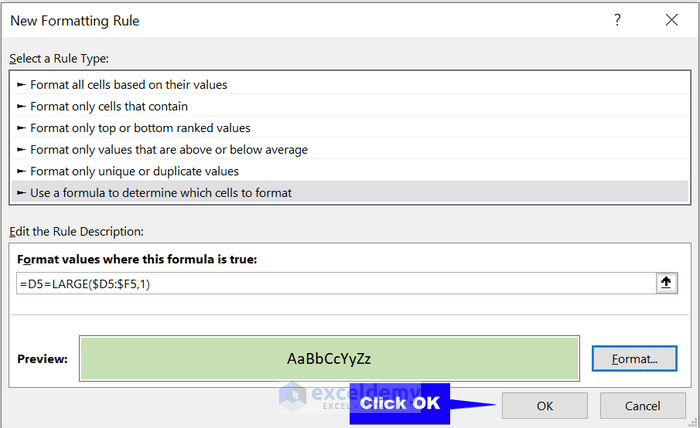
④ In the New Formatting Rule dialog box, select Use a formula to determine which cells to format. Enter the following formula:

This formula will return the 1st largest value of the three months. Click on Format.

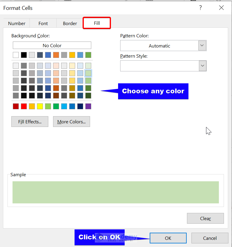
⑤  From the Format Cells dialog box, select Fill menu. Choose any fill colors. Click OK.

⑥  We have set our formula and fill color. Click on OK.

⑦ Check the Stop IF True checkbox. This is important as it will make sure that our formula will work only for rows independently. Click on New Rule to add more formulas.

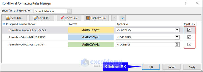
⑧ Create two more rules like the previous rule. These two rules will return 2nd and 3rd highest values respectively.

The formula for 2nd highest value is:

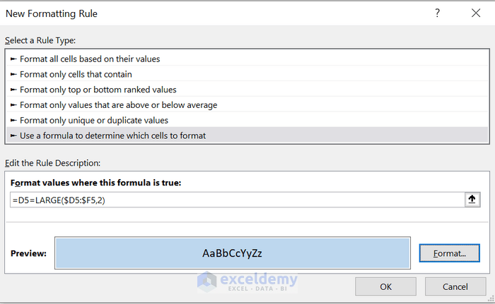
The formula for 3rd highest value is:

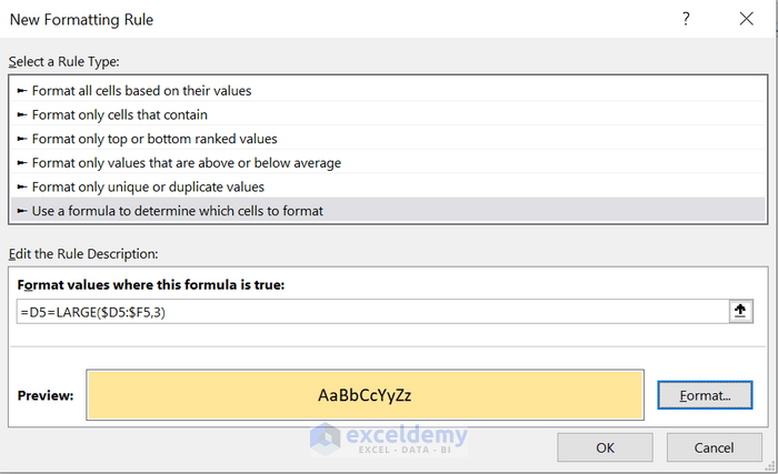
⑨ We have set all the formats and formulas. Remember to mark the checkboxes.

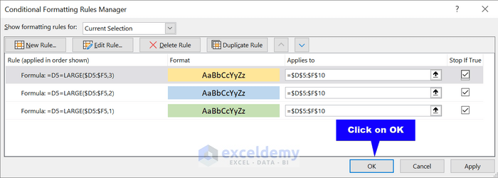
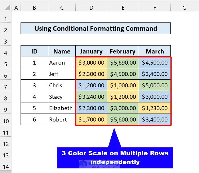
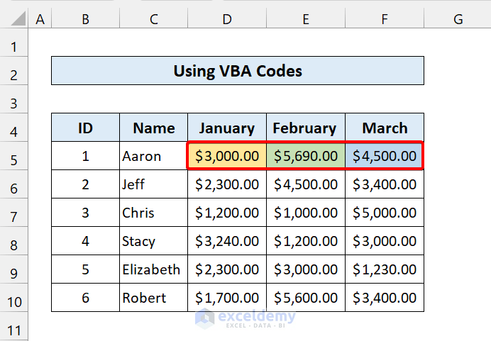
⑩ Click on OK. The desired output will be displayed as shown in the following image.

Read More: How to Apply Conditional Formatting to Multiple Rows

Method 2 – VBA codes for Multiple Rows Independently in Excel

Steps

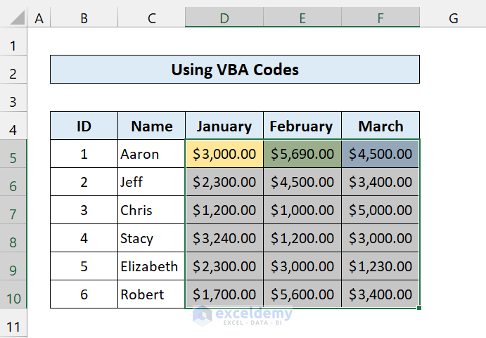
① Select the range of cells D5:F5.

② From the Home tab, go to Conditional Formatting > Manage Rules.

③ In the Conditional Formatting Rules Manager dialog box, click on New Rule.

④ In the New Formatting Rule dialog box, select Use a formula to determine which cells to format. Enter the following formula:

This formula will return the 1st largest value of the three months. Click on Format.

⑤  From the Format Cells dialog box, select Fill menu. Choose any fill colors. Click OK.

⑥  We have set our formula and fill color. Click on OK.

⑦ Check the Stop IF True checkbox.

⑧ Create two more rules following the steps for creating the first rule. These two rules will return 2nd and 3rd highest values respectively.

The formula for 2nd highest value is:

The formula for 3rd highest value:

⑨ We have set all the formats and formulas. Remember to check the checkboxes.

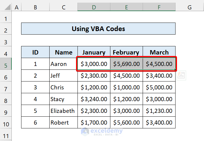
⑩ Click on OK. It will format the first row with 3 color scale.

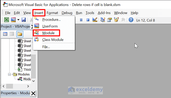
⑪ Press  Alt+F11  on your keyboard to open the VBA Editor. Select Insert > Module.

⑫ Enter the following code:

Sub format_all_rows()
Dim rng As Range
Dim r As Long
Set rng = Selection
rng.Rows(1).Copy
For r = 2 To rng.Rows.Count
  rng.Rows(r).PasteSpecial Paste:=xlPasteFormats
Next r
End Sub

⑬ Save the file. Select the range of cells D5:F10.

⑭ Press  Alt+F8  to open the Macro dialog box. Select format_all_rows.

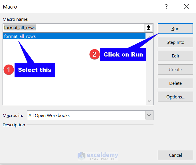
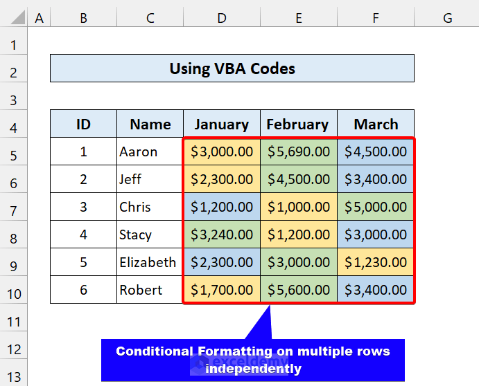
⑮ Click on Run. The output will display the dataset with conditional formatting on multiple rows independently as shown below.

Read More: How to Apply Conditional Formatting to Each Row Individually

Things to Remember

✎ To implement these methods, always check the “Stop If True” checkbox. It will ignore other rules when our data meet the conditions.

✎ This VBA code will generate the same rule for each row. So, if your dataset is large, it may slow down your process.

Download Practice Workbook

Related Articles

• Highlighting Row with Conditional Formatting Based on Date in Excel
• Conditional Formatting Based on Date in Another Cell in Excel
  
• How to Change Cell Color Based on Date Using Excel Formula
  
• How to Change Row Color Based on Text Value in Cell in Excel
• Excel Conditional Formatting for Dates within 30 Days
• Excel Conditional Formatting Based on Date
• Apply Conditional Formatting for Dates Older than Today
• Apply Conditional Formatting to Overdue Dates in Excel

<< Go Back to Conditional Formatting Rows | Conditional Formatting | Learn Excel