When you are working with a large database you may want to highlight some specific rows based on other cells or values to identify them quickly. In such a case, you can highlight rows using conditional formatting. Conditional formatting is a fascinating way to highlight a row and reduce your workload and it can improve your efficiency. Today in this article, we will demonstrate how to highlight rows using conditional formatting in Excel.
Highlight Row Using Conditional Formatting: 9 Suitable Methods
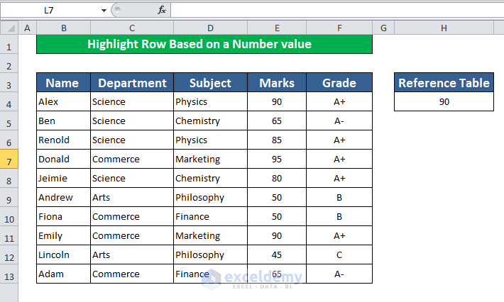
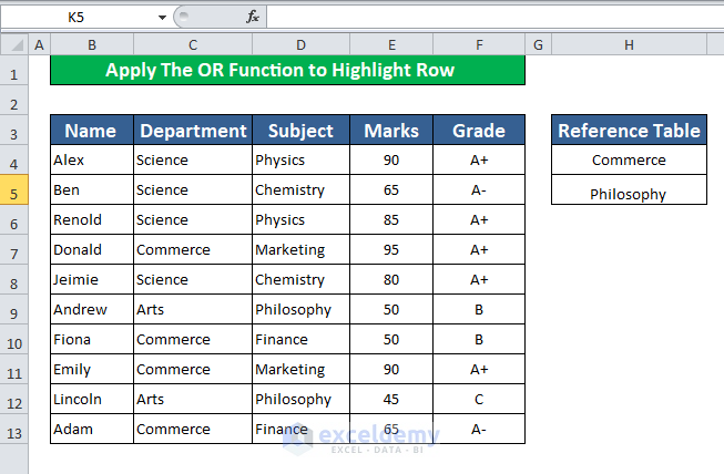
Think of a situation where you are given the Name, Department, Subject, Marks, and Grade of some students. Now you have to highlight some rows based on their names, departments, or grades using conditional formatting. In this section, we will demonstrate 9 different ways to do that.
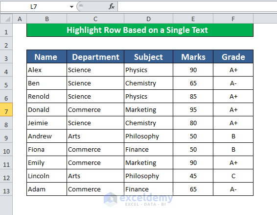
1. Highlight Row Based on a Single Text
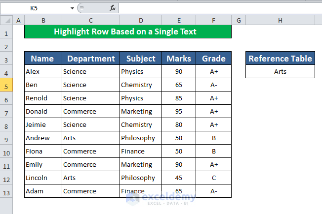
Highlighting rows based on a single text is one of the basic methods of conditional formatting. Suppose we have to highlight rows that have the Arts department. We will follow the steps below to learn.
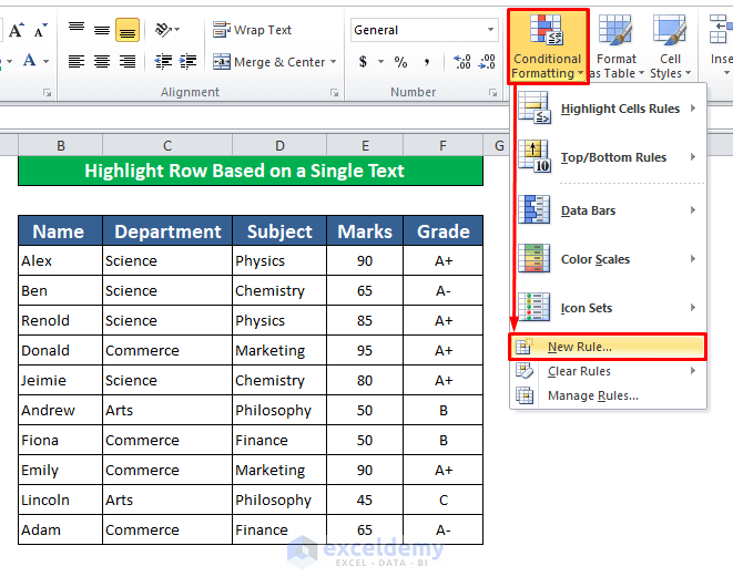
Step 1:
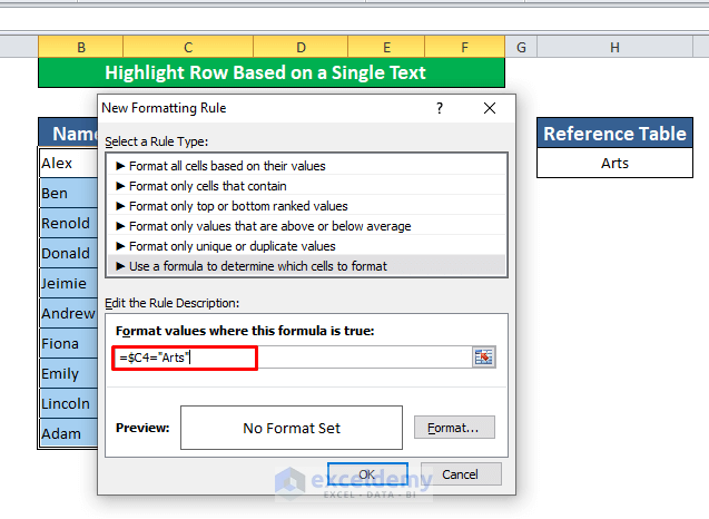
- Select the entire dataset. In your Home Tab, go to Conditional Formatting in the Style Group. Click on it to open available options and from them click on New Rule.
Home → Conditional Formatting → New Rule
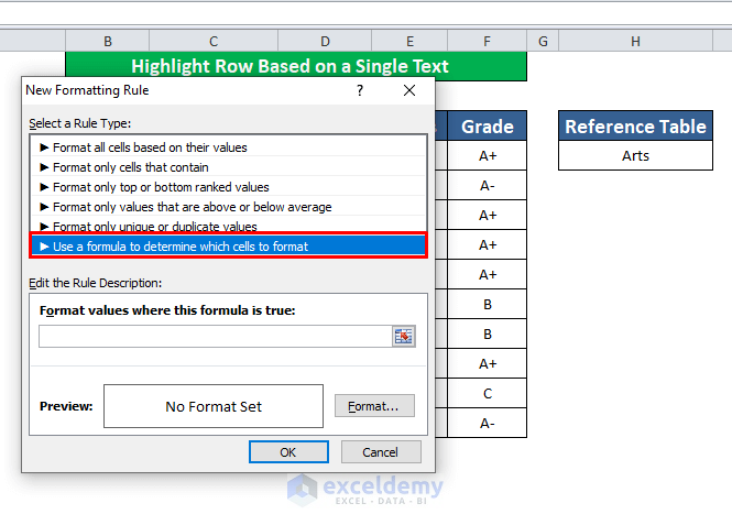
- A new window opens. Select Use a Formula to Determine the Cells to Format to continue.
Step 2:
- In the formula section, insert this formula.
=$C4="Arts"- This formula will compare the dataset cells with the name Arts. When the value will match, it will highlight the row.
Step 3:
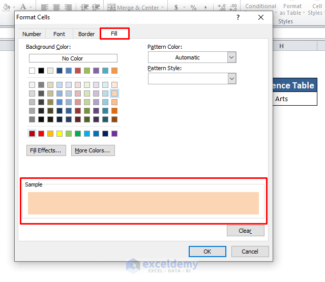
- We need to format the matched cells. The format section will help you out. We have chosen the color of the text Automatic. The fill cells option will help you to color the rows with a specific color. Choose any color you like to go.
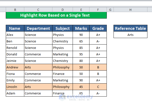
- Now that we have completed all the actions, click OK to get the result.

- We have highlighted our rows based on a text value in a cell using conditional formatting.
Read More: How to Change a Row Color Based on Text Value in Cell in Excel
2. Highlight Row Using Different Color Based on Multiple Texts
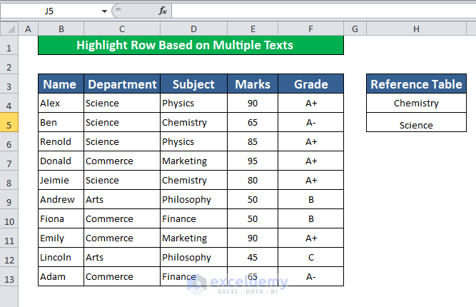
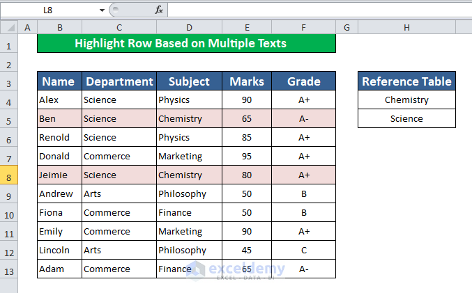
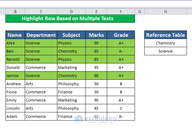
Following the same instructions as discussed in the previous method, we can highlight rows based on multiple conditions. Consider a case where you have to highlight the rows that have the Chemistry subject and Science department in them. Follow the steps below to learn this technique.
Step 1:
- Go to the New Formatting Window following these steps.
Home → Conditional Formatting → New Rule
- Select Use a Formula to Determine the Cells to Format.
- Write down the formula to specify the cells that contain the Chemistry The Formula is,
=$D4="Chemistry"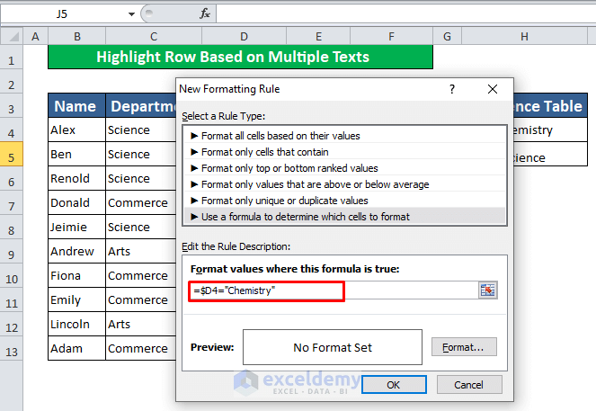
- Select the color format for your matched cells. Click OK to continue
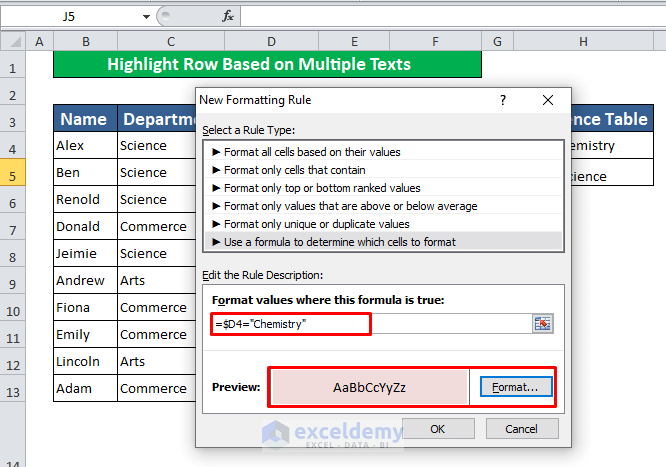
- The conditional formatting features successfully highlight the rows.
Step 2:
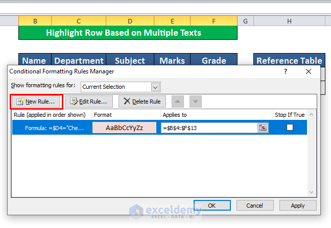
- Now we need to highlight the rows that contain the Science department in them. For that, go to
Home → Conditional Formatting → Manage Rules
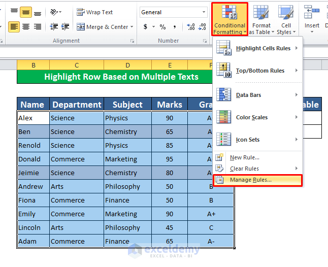
- The Conditional Formatting Rules Manager window appears. Click New Rule to add another one.
Step 3:
- Set the formula for the second condition. Write down the formula in the formula box.
=$C4="Science"- Set the format and you are good to go.
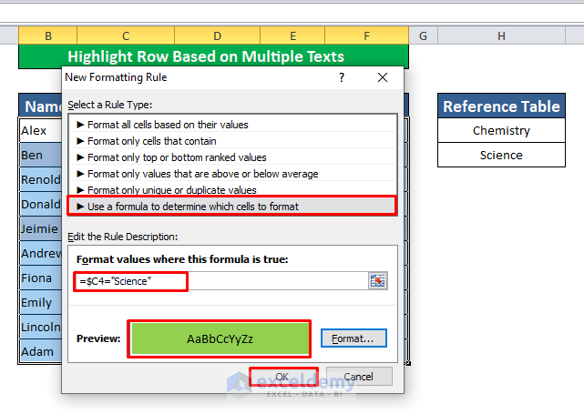
- Finally, click OK to highlight row based on multiple conditions using conditional formatting
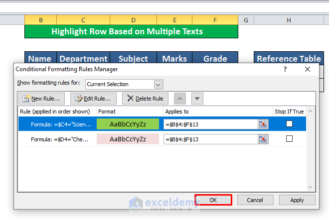
- The result is here.
Read More: Applying Conditional Formatting for Multiple Conditions in Excel
3. Highlight Row with Conditional Formatting Based on a Number value
We can highlight a row using conditional formatting based on numbers too. In this given situation, we have to highlight the rows with a mark equal to 90.
Step 1:
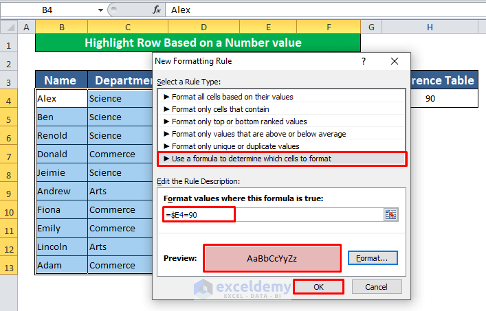
- Insert the formula in the formula box of the New Formatting Rule
=$E4=90- Specify the formatting and click OK to continue.
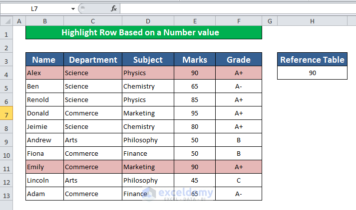
- Our job here is done.
Step 2:
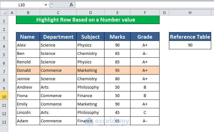
- Using the same procedures, you can also apply the greater than or the less than conditions. For highlighting row having a number greater than 90, the formula is,
=$E4>90- Confirm the format and click OK.

- We have got the result. In the same way, you can find the number less than 90.
Read more: How to Apply Conditional Formatting to Multiple Rows
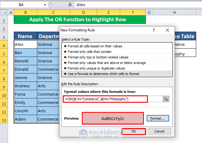
4. Apply The OR Function to Highlight Row
You can use The OR Function to apply conditional formatting. We want to highlight the Commerce department or Philosophy subject using the OR function. Insert those texts into your reference table.
Step 1:
- Write down the OR formula in the formula box. The Formula is,
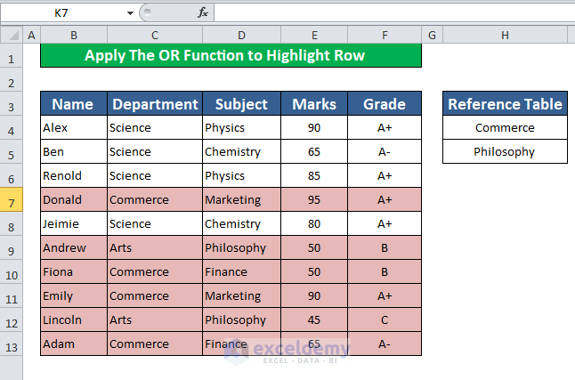
=OR($C4="Commerce",$D4="Philosophy")- The OR formula will compare the cell values with Commerce and Philosophy and then it will color the rows that matched the conditions.
Step 2:
- Select a formatting style according to your preferences.
- Click OK and your job is done.
Read More: Excel Conditional Formatting Formula with IF
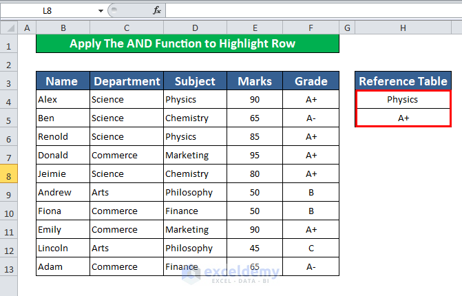
5. Insert The AND Function to Highlight Row with Conditional Formatting
The AND Function also helps you to highlight rows using conditional formatting. Here we will apply a new condition. We will change row colors that have both Physics and A+ grades in them.
Step 1:
- Following the same procedures discussed above, go to the New Formatting Rule window and apply the AND formula is,
=AND($D$4="Physics",$F4="A+")- Set the formatting styles and click OK to format the cells.
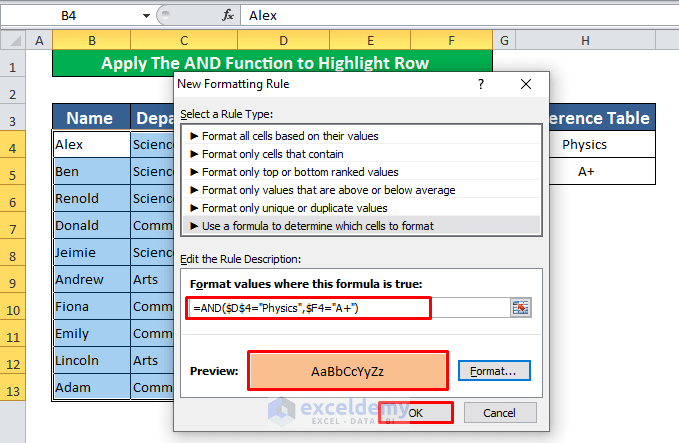
- We have successfully highlighted the rows according to the conditions.

Read More: How to Apply Conditional Formatting to Each Row Individually
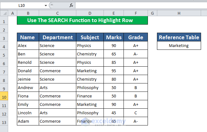
6. Use The SEARCH Function to Highlight Row
You can Use The SEARCH Function to find and highlight any specific rows in your dataset using conditional formatting. To do this, insert a name that you want to find in the database.
Step 1:
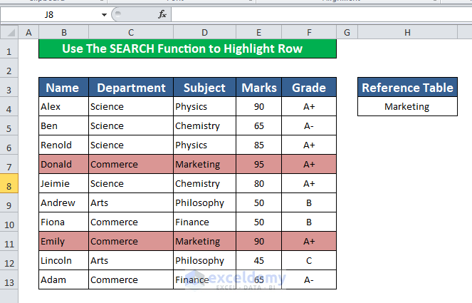
- Apply the SEARCH function to find Marketing. The formula is,
=SEARCH($H$4,$D4)>0- Click OK to continue.
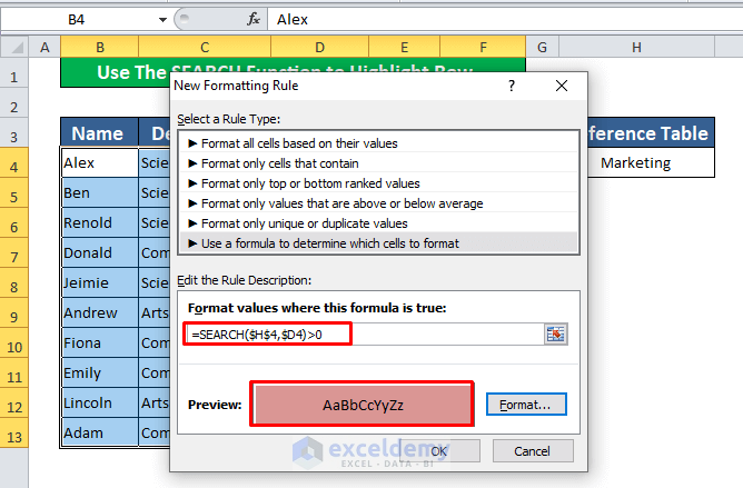
- See, we have highlighted the rows that contain the subject Marketing.
Read More: Conditional Formatting on Multiple Rows Independently in Excel
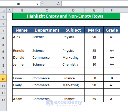
7. Highlight Empty and Non-Empty Row with Conditional Formatting
Sometimes you have empty rows in your database that you want to highlight. You can do it easily using conditional formatting.
Step 1:
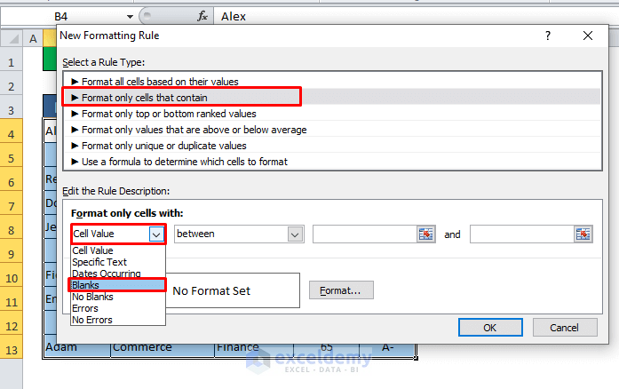
- Open the New Formatting Rule window and select Format Only the Cells that Contain
- Select Blank from the options
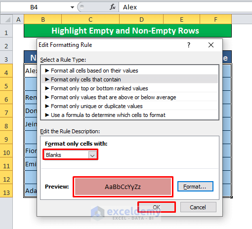
- Set the Formatting and click OK to continue
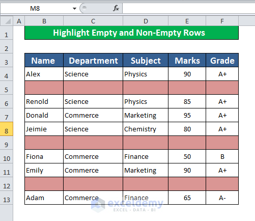
- The blank cells are now highlighted with color.
Read More: How to Apply Conditional Formatting for Blank Cells in Excel
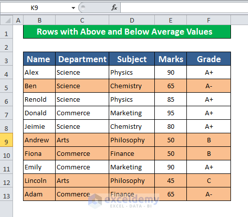
8. Conditional Formatting to Highlight Row with Above and Below Average Values
Step 1:
- In order to find above or below average values from your dataset, apply this formula,
=$E4<AVERAGE($E$4:$E$13)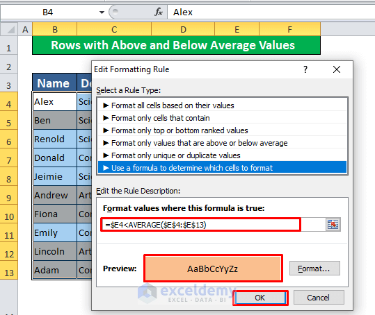
- OK to get the result. That’s how you can find below or above-average values.
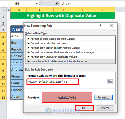
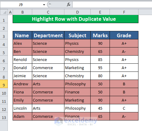
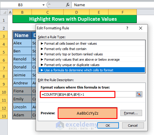
9. Highlight Rows with Duplicate Value Using Conditional Formatting
In some cases, you need to highlight rows with duplicate values in them. The COUNTIF function can help you in this situation. Follow these instructions to learn this method.
Step 1:
- Apply this formula in the formula box.
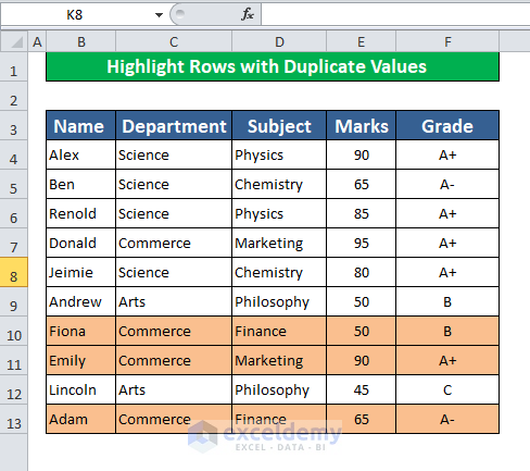
=COUNTIF($E$4:$E$13,$E4)>1- Here $E$4:$E$13 is the range and $E4 is the criteria. If the function finds a value of more than once, it will highlight the row.
- OK to get the result. This result here is achieved with the first occurrence.
Step 2:
- We can also highlight duplicate rows without the first occurrence. For that, the formula is,
=COUNTIF($E$4:$E4,$E4)>1- Set the format and get the result by clicking OK.
- The final result is here.
Things to Remember
👉 When you want to find out case sensitive name, you can use the FIND function instead of the SEARCH function.
👉 Use the Absolute Cell references ($) to block the cells.
Download Practice Workbook
Download this practice book to exercise the task while you are reading this article.
Conclusion
We have discussed nine suitable ways to highlight rows using conditional formatting in Excel. You are most welcome to comment if you have any questions or queries. You can also check out our other articles related to the Excel tasks!
Similar Articles to Explore
- Excel Conditional Formatting Based on Date
- Highlighting Row with Conditional Formatting Based on Date in Excel
- Conditional Formatting Based on Date in Another Cell in Excel
- Apply Conditional Formatting for Dates Older Than Today in Excel
- How to Change Cell Color Based on Date Using Excel Formula
- Apply Conditional Formatting to Overdue Dates in Excel
- Excel Conditional Formatting for Dates within 30 Days
<< Go Back to Conditional Formatting Rows | Conditional Formatting | Learn Excel
Get FREE Advanced Excel Exercises with Solutions!
