This is an overview:
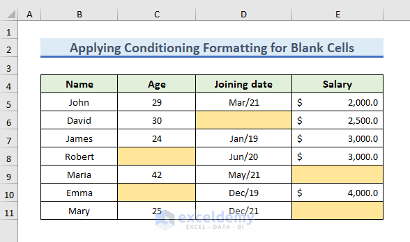
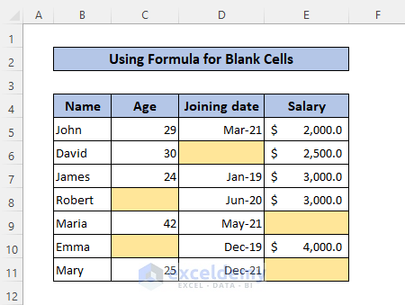
This is the sample dataset.

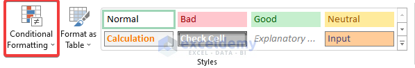
Method 1 – Using the Conditional Formatting Command
This is the Conditional Formatting command:
1.1 Use the Built-in Formatting Rule in the Conditional Formatting Option
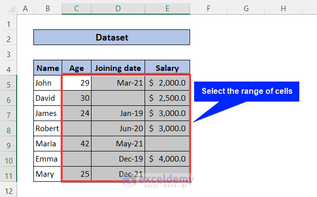
Steps
- Select the entire dataset. Here, C5:E11.
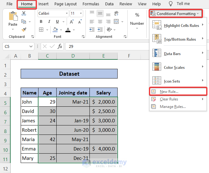
- In the Home tab, go to Conditional Formatting >> New Rule.
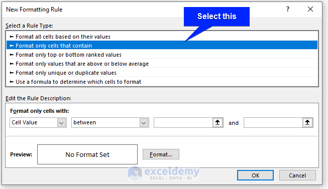
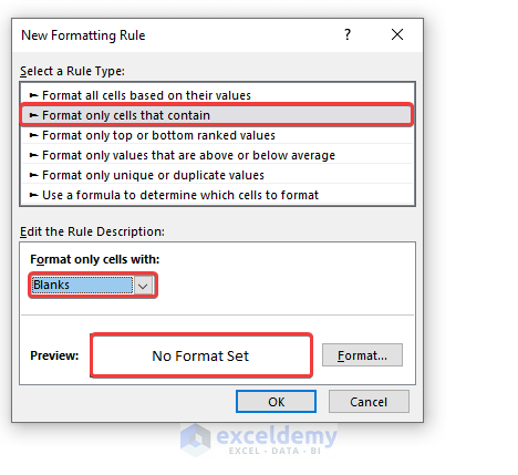
- In New Formatting Rule, select Format only cells that contain.
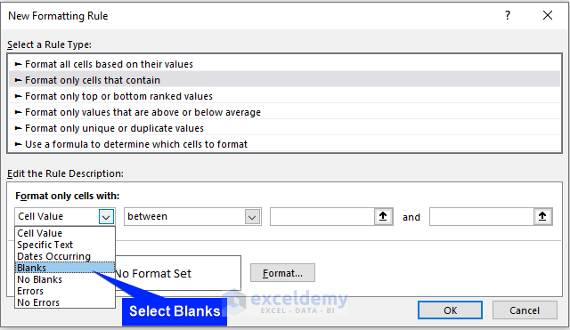
- Select Blanks.
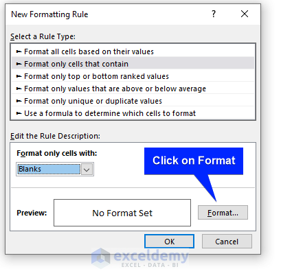
- Click Format.
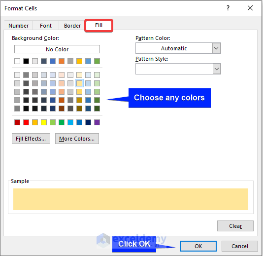
- Select Fill.
- Choose a color and click OK.
Formatting is set.
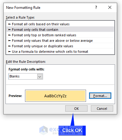
- Click OK.

1.2 Apply Conditional Formatting using a Formula
Steps
- Select the entire dataset. Here, C5:E11.
- In the Home tab, go to Conditional Formatting >> New Rule.
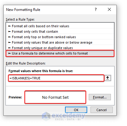
- In New Formatting Rule, select Use a formula to determine which cells to format.
- Enter the following formula:
=ISBLANK(C5)=TRUE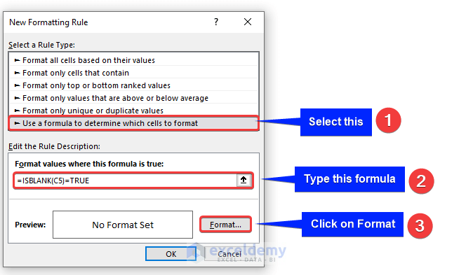
- Click Format.
- Select Fill.
- Choose a color and click OK.
Formatting is set.
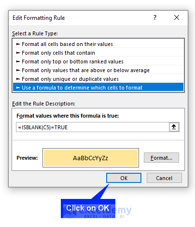
- Click OK.
Read More: Conditional Formatting If Cell is Not Blank
Method 2 – Using a VBA Code to Apply Conditional Formatting to Blank Cells
Steps
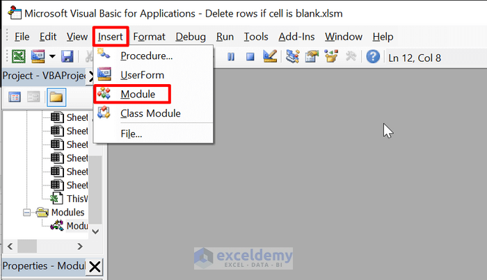
- Press Alt+F11 to open the VBA editor.
- Select Insert >> Module.
- Use the following code in the module:
Sub format_blank_cells()
Dim range_of_cells As Range
Set range_of_cells = Selection
range_of_cells.SpecialCells(xlCellTypeBlanks).Interior.Color = vbBlue
End Sub- Save the file.
- Select C5:E11.

- Press Alt+F8 to open the Macro dialog box.
- Select format_blank_cells.
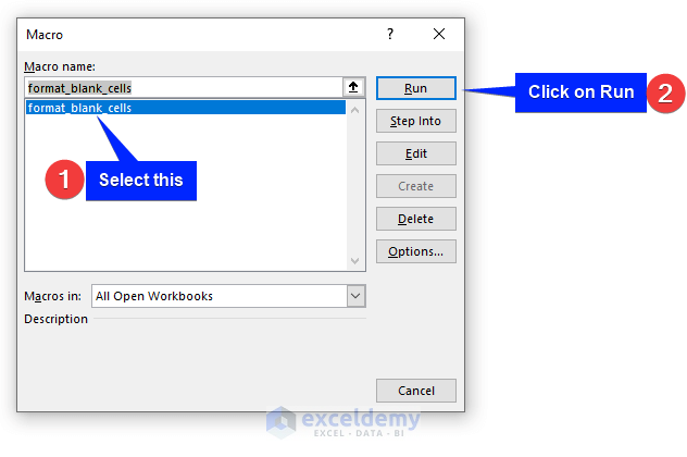
- Click Run.

Read More: Apply Conditional Formatting to Each Row Individually
Skip Conditional Formatting for Blank Cells in Excel
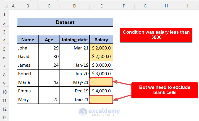
Conditional formatting was used to highlight cells with values less than 3000 in the Salary column. Blank cells were also formatted.
Steps
- Select E5:E11.

- In the Home tab, go to Conditional Formatting >> New Rule.
- Choose one of the previous methods to format blank cells.
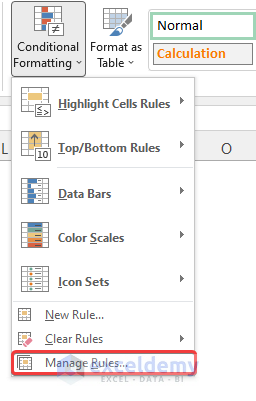
- In the Home tab, go to Conditional Formatting >> Manage Rules.
- In the Conditional Formatting Rules Manager window, check the boxes shown below.
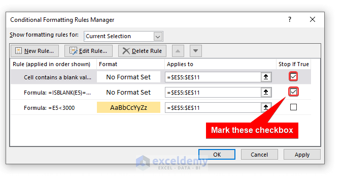
- Click OK.

Read More: How to Remove Conditional Formatting but Keep the Format in Excel
How to Undo Conditional Formatting in Blank Cells in Excel
1. Use the Quick Analysis option
Steps
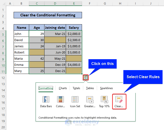
- Select the cell range.
- Click the Quick Analysis option at the right bottom corner.
- Select Clear Rules.
It will remove conditional formatting from blank cells.
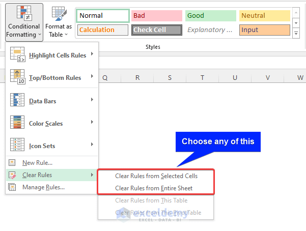
2. Using the Conditional Formatting Command
- Go to Conditional Formatting >> Clear Rules.
- Choose an option.
Download Practice Workbook
Download the practice workbook
Related Articles
- How to Apply Different Types of Conditional Formatting in Excel
- How to Find External Links in Conditional Formatting in Excel
- How to Apply Conditional Formatting on Multiple Columns in Excel
- How to Compare Two Columns Using Conditional Formatting in Excel
- How to Remove Conditional Formatting in Excel
- How to Do Conditional Formatting in Excel
- Conditional Formatting with Formula in Excel
<< Go Back to Conditional Formatting | Learn Excel
Get FREE Advanced Excel Exercises with Solutions!
