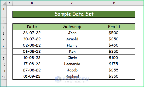
Consider the following dataset.
Example 1 – Highlight Cells Rules
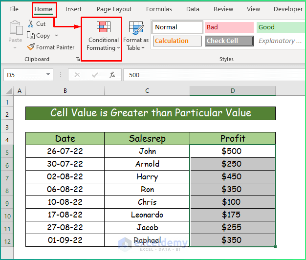
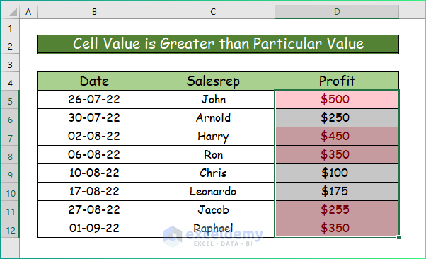
1.1 The Cell Value Is Greater Than a specified Value
Step 1:
- Select D5:D12.
- In the Home tab, select Conditional Formatting.
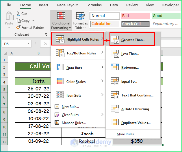
Step 2:
- Choose Highlight Cells Rules.
- Choose Greater Than.
Step 3:
- In the Greater Than dialog box, set a value. Here, highlight values greater than 250.
- Click OK.
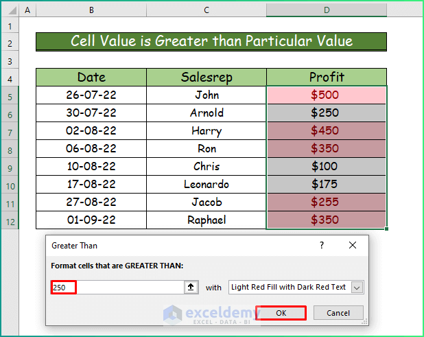
Step 4:
This is the output.
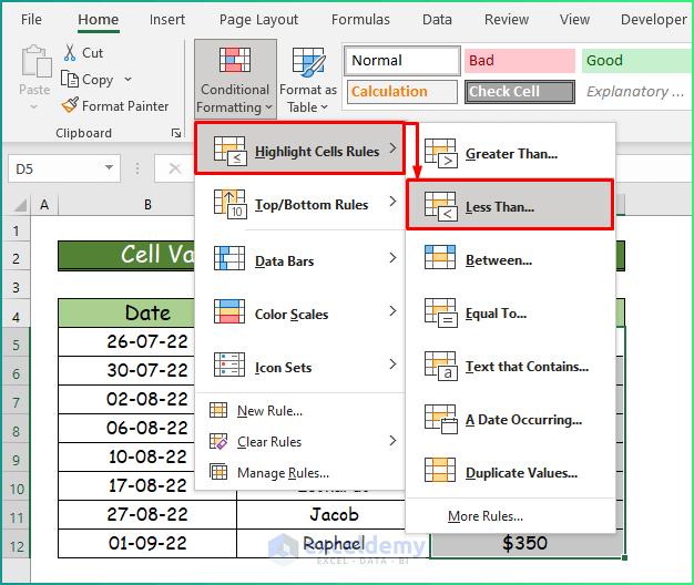
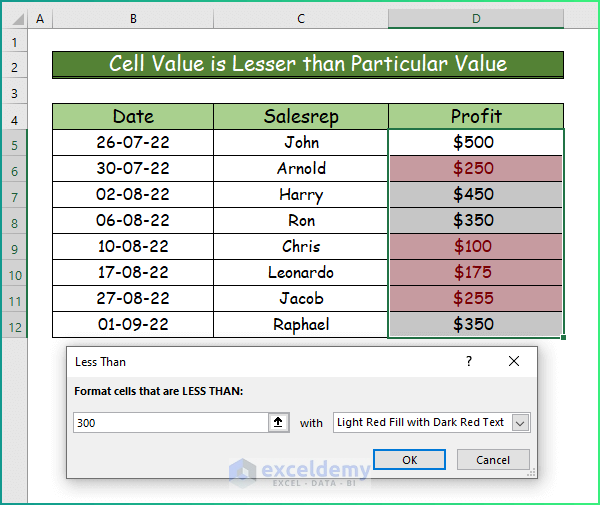
1.2 Cell Values Less Than a specified Value
Step 1:
- Select the cell range.
- Go to Highlight Cells Rules.
- Choose Less Than.
Step 2:
- Set a value. Here, highlight values less than 300.
- Click OK.
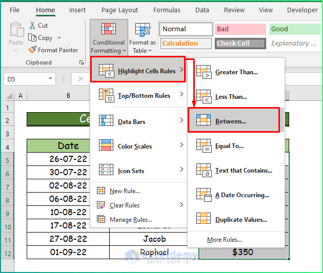
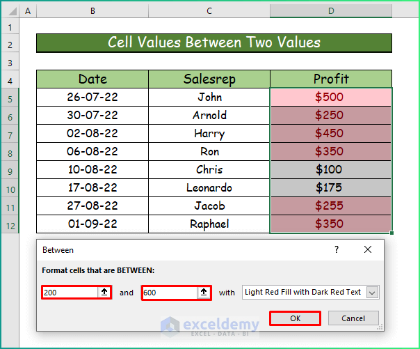
1.3 Cell Values Between Two Values
Step 1:
- Choose Between in Highlight Cells Rules.
- Select D5:D12.
Step 2:
- Set two values. Here, highlight values between 200 and 600.
- Click OK.
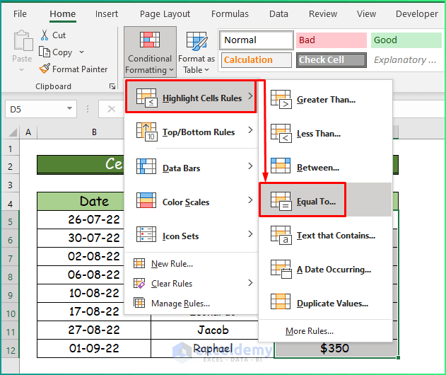
1.4 The Cell Value Is Equal to a specified Value
Step 1:
- Select D5:D12.
- Choose Equal To in Highlight Cells Rules.
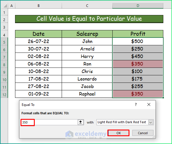
Step 2:
- Set a value. Here, highlight values equal to 350.
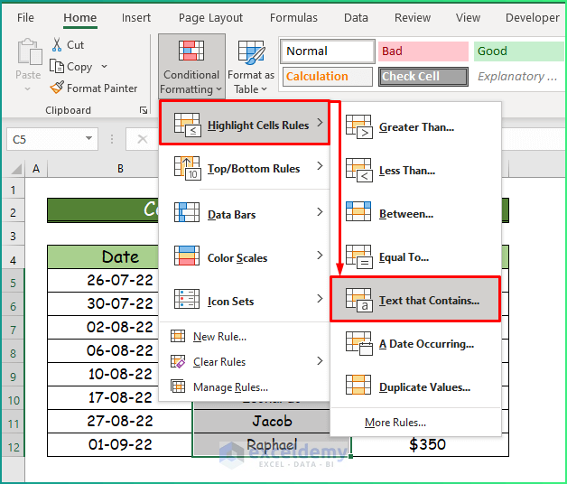
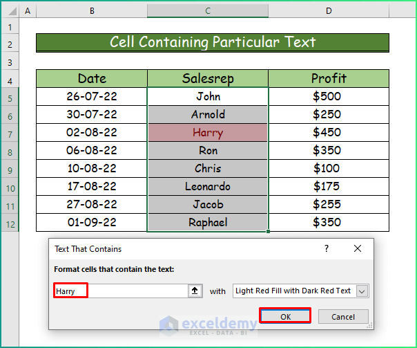
1.5 Cell Containing a specific Text
Step 1:
- Select C5:C12.
- Choose Text that Contains in Highlight Cells Rules.
Step 2:
- In Text that Contains, enter a text in the dataset.
- Click OK.
Read More: Excel Conditional Formatting Formula If Cell Contains Text
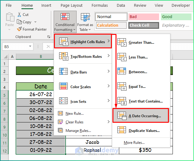
1.6 Cells Containing specific Dates
Step 1:
- Select B5:B12.
- In Highlight Cells Rules, choose A Date Occurring.
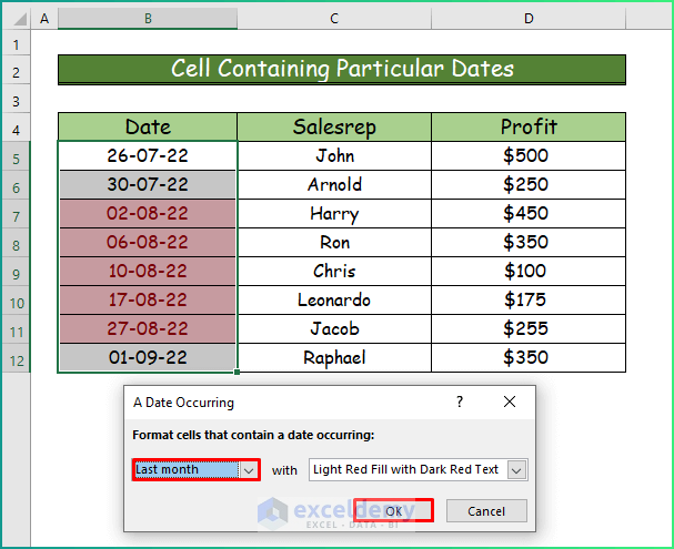
Step 2:
- Set the rule: dates in the previous month.
This is the output.
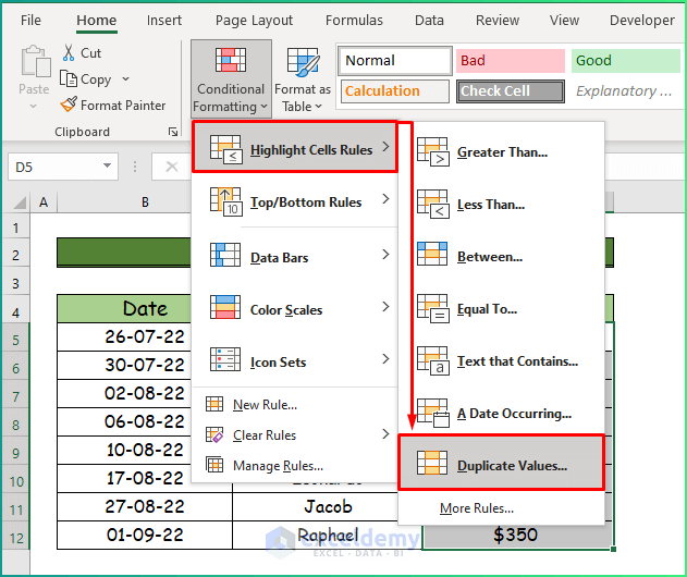
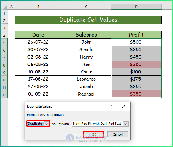
1.7 Duplicate Cell Values
Step 1:
- Select the cell range.
- Choose Duplicate Values.
Step 2:
Duplicate values are automatically highlighted.
Read More: Excel Conditional Formatting Based on Date
Example 2 – Top and Bottom Rules
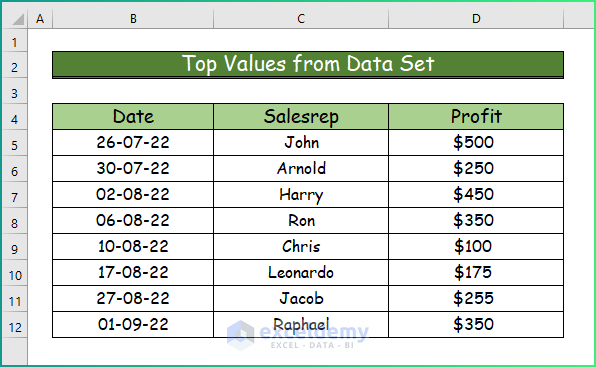
2.1 Top Values from the Dataset
Step 1:
Consider the following dataset:
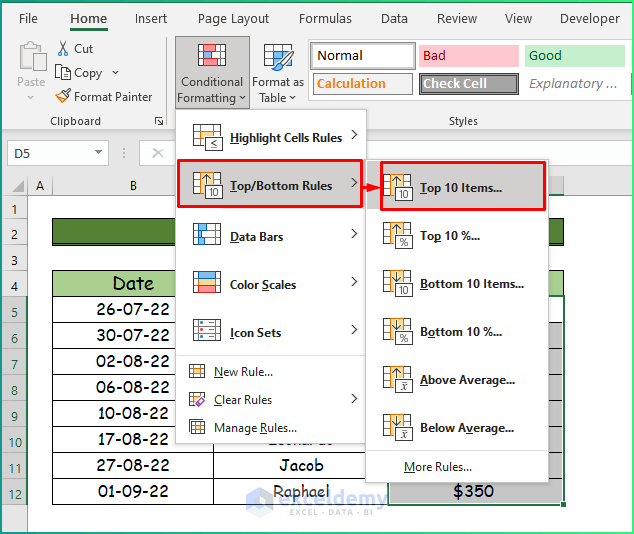
Step 2:
- Select D5:D12.
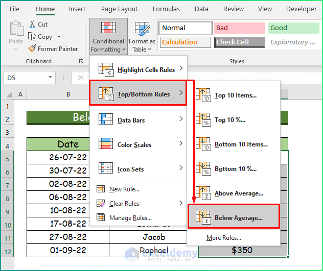
- In the Home tab, choose Top/Bottom Rules in Conditional Formatting.
- Select Top 10 Items.
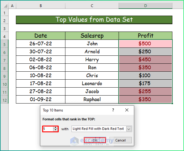
Step 3:
- Enter the top values. (As this dataset contains less than 10 items, the top 5 values will be highlighted).
This is the output.
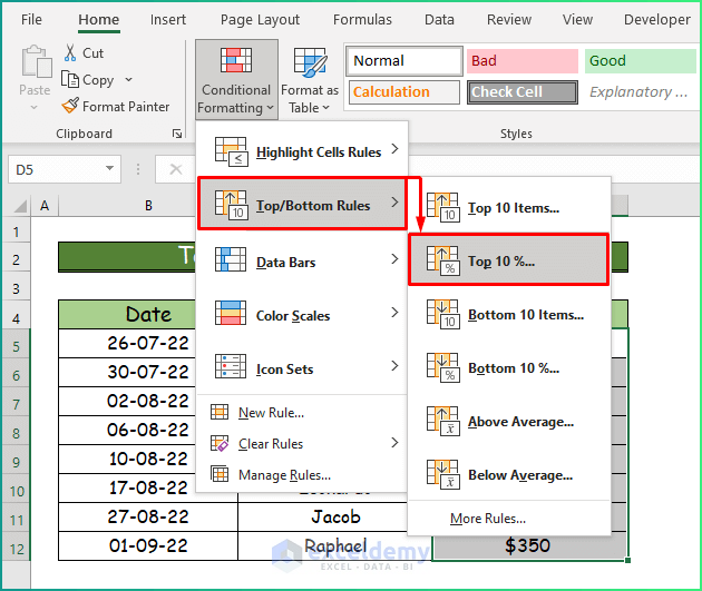
2.2 Top 10% Values in the Dataset
Step 1:
- Select D5:D12.
- Choose Top 10% in Top/Bottom Rules.
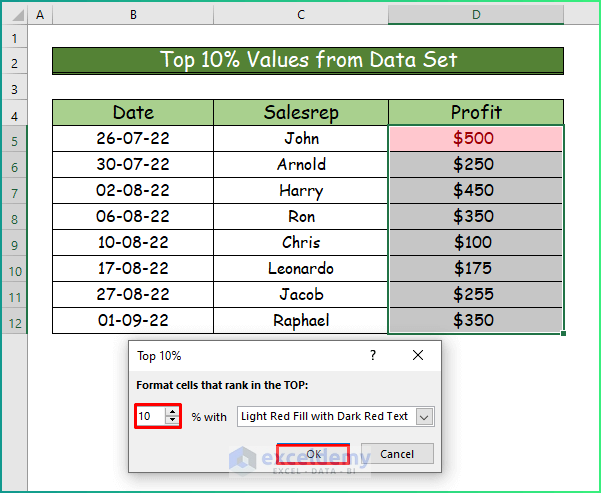
Step 2:
- Set the condition: cells in the top 10% of the total value.
This is the output.
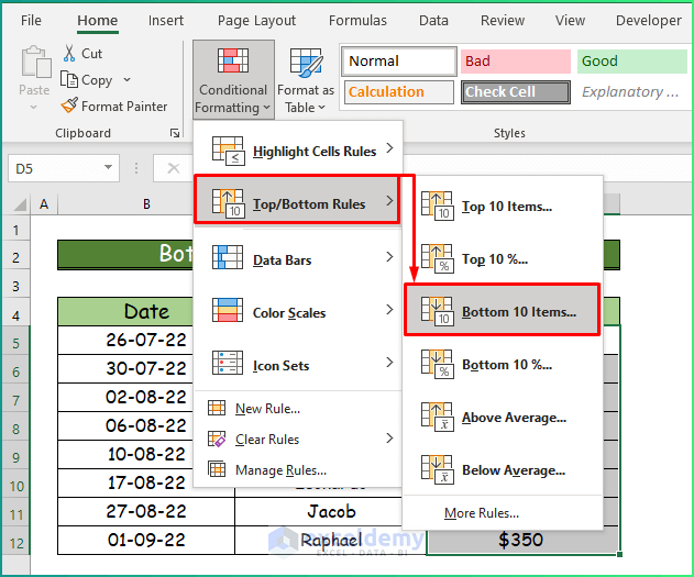
2.3 Bottom Values from the Dataset
Step 1:
- Select the data range.
- Choose Bottom 10 Items.
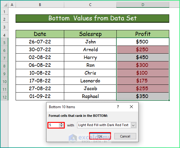
Step 2:
- Set the number of bottom values to be shown.
This is the output.
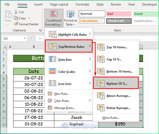
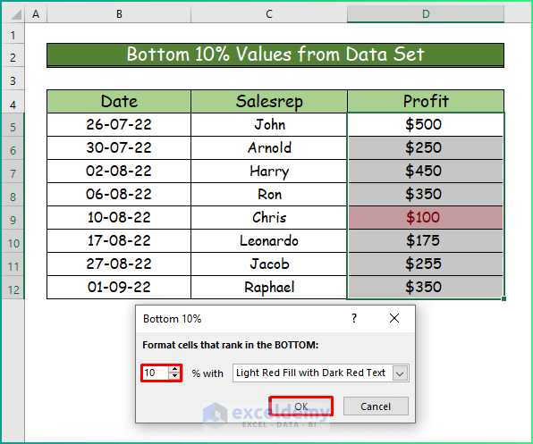
2.4 Bottom 10% Values from the Dataset
Step 1:
- Select the dataset.
- Go to Top/Bottom Rules and choose Bottom 10%.
Step 2:
- Set a percentage.
Values matching the criterion will be highlighted: here, $100.
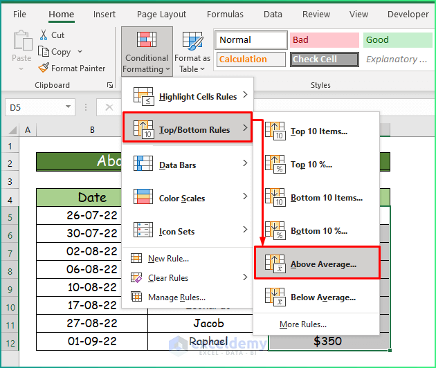
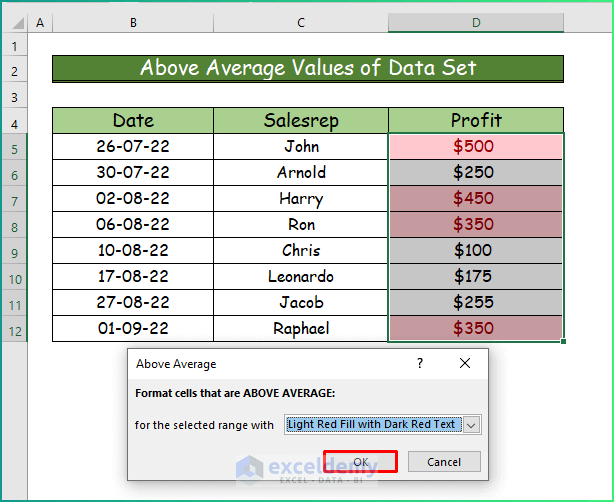
2.5 Above Average Values in the Dataset
Step 1:
- Select the cell range.
- Select Above Average in Top/Bottom Rules.
Step 2:
Values will automatically be highlighted .
2.6 Below the Average Values in the Dataset
Step 1:
- Select the data range.
- Go to Below Average.
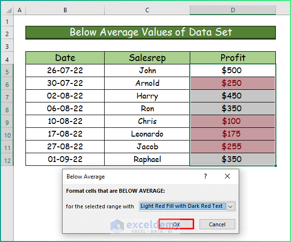
Step 2:
This is the output.
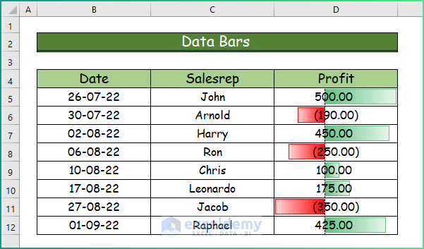
Example 3 – Data Bars
Step 1:
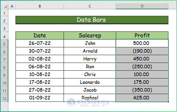
Consider the following dataset. The profit column has negative values:
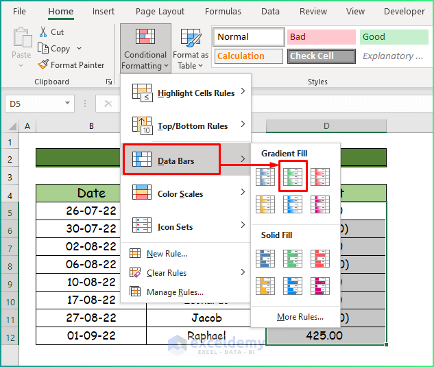
Step 2:
- In Conditional Formatting, select Data Bars.
- Choose an option.
Step 3:
This is the output. Positive values are highlighted in green and negative values are displayed in red.
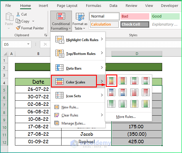
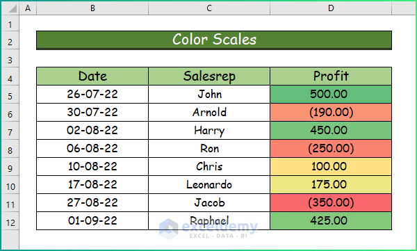
Example 4 – Color Scales
Step 1:
- Select the data range and go to Color Scales in Conditional Formatting.
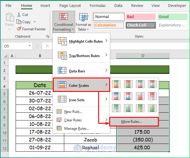
Step 2:
- In Color Scales, select More Rules.
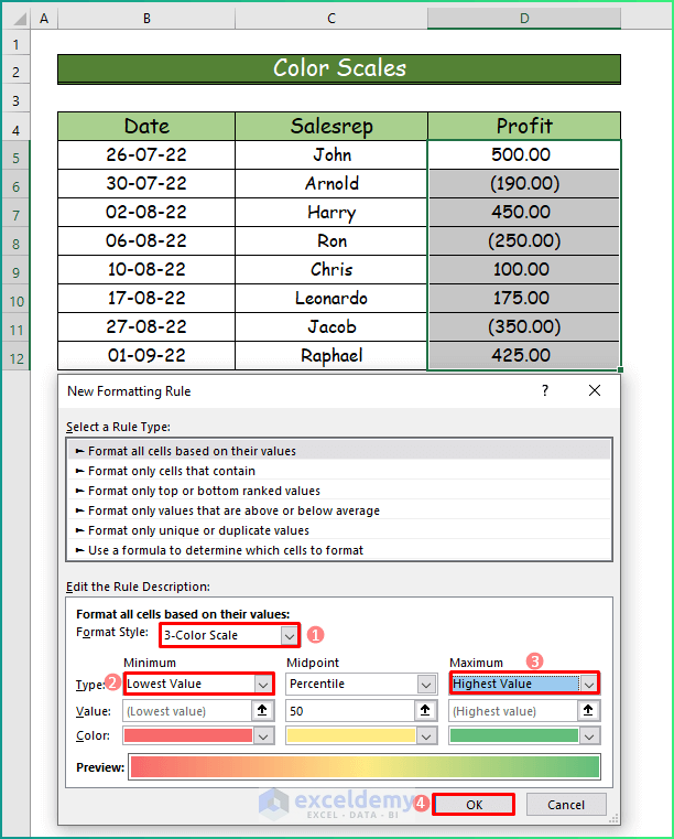
Step 3:
- Choose 3-Color Scale in Format Style.
- In the Type box, select Lowest Value in Minimum and Highest Value in Maximum. Lower values will have a red color scale, middle values will have a green color scale and higher values will have a green color scale.
- Click OK.
Step 4:
This is the output.
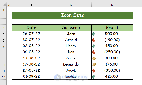
Example 5 – Icon Sets
Step 1:
- Select the data range.
- Select Icon Sets in Conditional Formatting.
- Choose an option.

Step 2:
This is the output. Red icons represent the lower values, yellow icons represent the middle values, and green icons represent the higher values in the dataset.
Download Practice Workbook
Download the free Excel workbook.
Related Articles
- How to Find External Links in Conditional Formatting in Excel
- How to Apply Conditional Formatting for Blank Cells in Excel
- How to Apply Conditional Formatting on Multiple Columns in Excel
- How to Compare Two Columns Using Conditional Formatting in Excel
- How to Remove Conditional Formatting in Excel
- How to Remove Conditional Formatting but Keep the Format in Excel
- Conditional Formatting with Formula in Excel
<< Go Back to Conditional Formatting | Learn Excel
Get FREE Advanced Excel Exercises with Solutions!
