How to Apply Conditional Formatting Formula in Excel If Cell Contains Text (6 Methods)

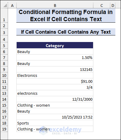
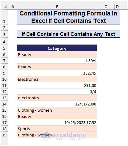
Method 1 – Highlight Cells Containing Any Text

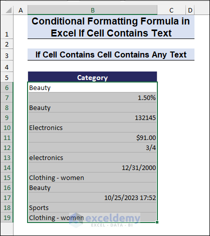
• Select the cells where you want to apply conditional formatting.

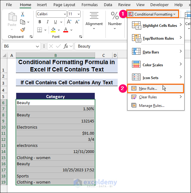
• Go to the Styles group and click Conditional Formatting.
• Choose New Rule. 

• Select Use a formula to determine which cells to format.
• Enter the formula:

• • Where B6 is the first cell in the range.

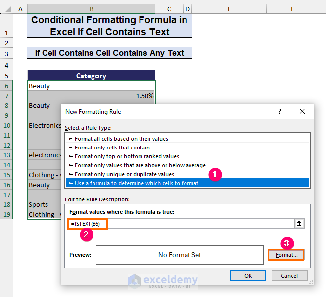
• Customize the formatting (e.g., fill color) in the Format Cells dialog.
• Confirm to apply the conditional formatting.

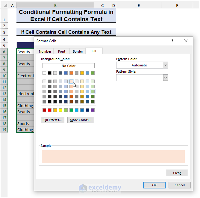
• A Format Preview will appear.
• Click OK to apply the Conditional Formatting.

• We will get the highlighted cells with conditional formatting containing the text values only.

Read More: Conditional Formatting Multiple Text Values in Excel

Method 2 – Highlight Cells with Specific Text

• Similar to Method 1, use the New Rule dialog.
• Enter the formula:

• • Where G6 contains your specific lookup value.
• Apply formatting as desired.

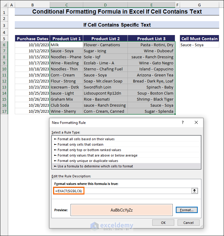
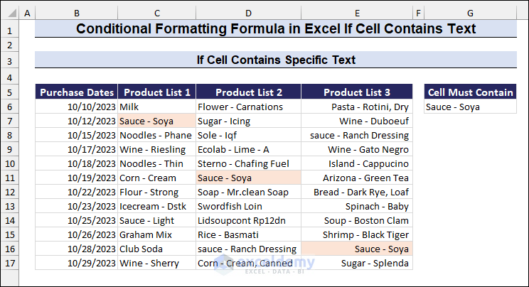
• This method helps find exact matches (e.g., Sauce – Soya) in your dataset.

Read More: Applying Conditional Formatting for Multiple Conditions in Excel

Method 3 – Case-Sensitive Text Highlighting

• Use the New Rule dialog.
• Enter the Formula:

• • Where G6 is your lookup value.
• Click on Format to apply the formatting as before.
• After selecting the desired format, click OK to apply.

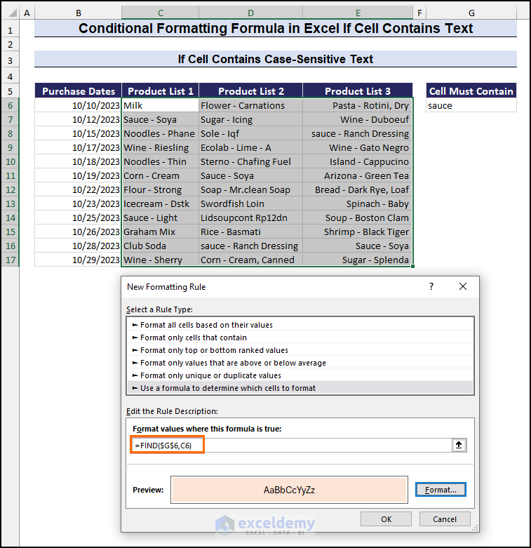
• This method differentiates case-sensitive matches.

Method 4 – Partial Matched Text Highlighting

• We’ll use the SEARCH function to highlight cells containing partially matched text.
• The SEARCH function is case-insensitive and finds matches partially or fully.
• Example: Suppose we want to highlight cells containing wine.
  • Enter the formula in the Format values where this formula is true box:

• Apply the desired formatting and click OK.

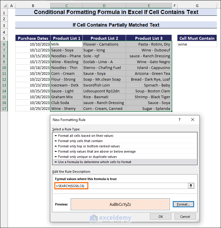
• The cells will be highlighted based on partial matches (e.g., sauce, corn).

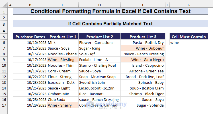
• The SEARCH function ignores case sensitivity.
• You can see in the below GIF that the cells are highlighted according to the value in cell G6 (e.g., sauce, corn). It is irrespective of the case, as the SEARCH function is not case-sensitive.

Method 5 – OR Logic for Multiple Text Strings

• We’ll highlight cells matching any of the values in cells G6 and G7 (e.g., Sauce or Wine).
• Use a formula combining IF, OR, ISNUMBER, and SEARCH functions:
• Enter the following formula in the Format values where this formula is true box:

• Apply formatting and click OK.

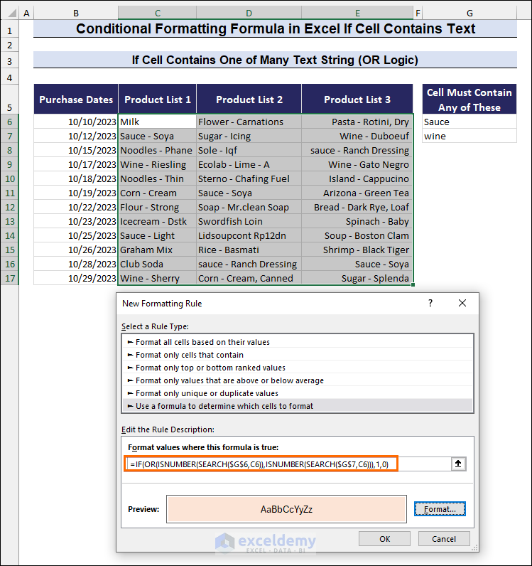
• The cells will be highlighted if they match either Sauce or Wine.

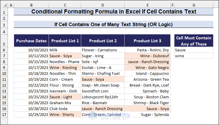
• You can see in the below GIF that the cells are highlighted according to the values in cells G6, change the values in G6 and G7, and get all the highlighted values for any of the matches.

Read More: Excel Conditional Formatting Formula with IF

Method 6 – AND Logic for Multiple Text Strings

• Similar to Method 5, but we’ll highlight cells matching both criteria in cells G6 and G7 (e.g., Sauce and Soya).
• Use a formula combining IF, AND, ISNUMBER, and SEARCH functions:
• Enter the following formula in the Format values where this formula is true box:

• Apply formatting and click OK.

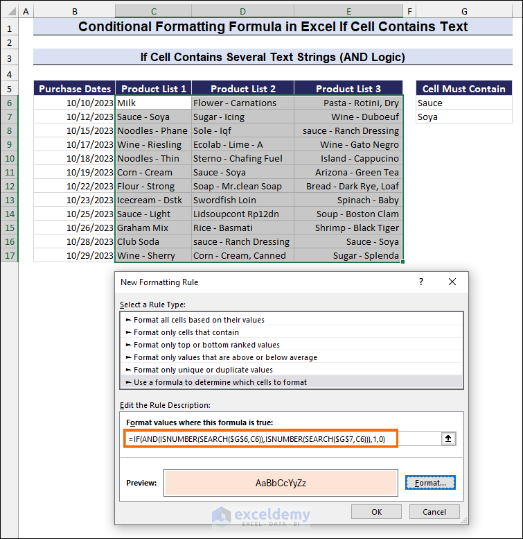
• The cells will be highlighted if they contain both Sauce and Soya.

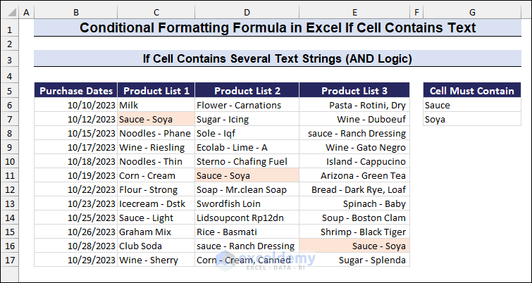
• You can see in the below GIF that the cells are highlighted according to the values in cells G6 and G7. Change the values in G6 and G7 and get all the highlighted values for both matches.

Download Practice Workbook

You can download the practice workbook from here:

Related Articles

• How to Format Cell Based on Formula in Excel
• How to Use Conditional Formatting Based on VLOOKUP in Excel
• How to Apply Conditional Formatting with INDEX-MATCH in Excel
• Conditional Formatting If Cell is Not Blank
• How to Change Text Color Based on Value with Excel Formula
  
• Conditional Formatting Entire Column Based on Another Column in Excel
• Excel Highlight Cell If Value Greater Than Another Cell

<< Go Back to Conditional Formatting Formula | Conditional Formatting | Learn Excel