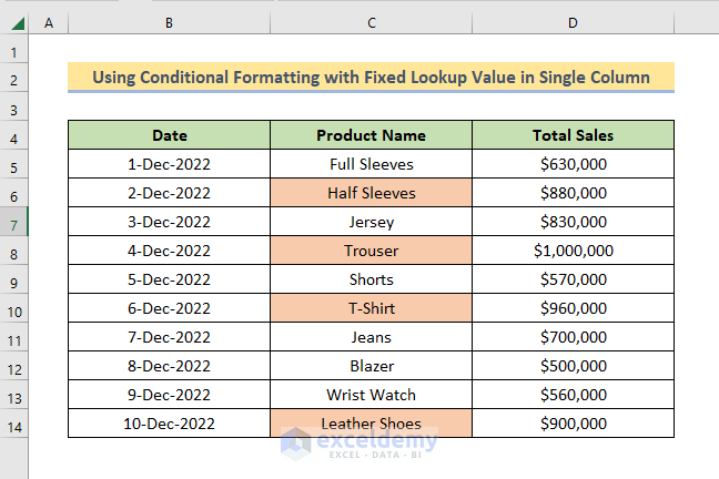
Method 1 – Using Conditional Formatting with INDEX-MATCH with a Fixed Lookup Value in Excel (Over a Single Column)
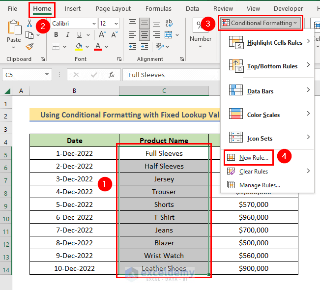
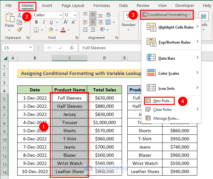
- Select the column on which you want to apply Conditional Formatting.
- We selected the column Product Name (C5:C14).
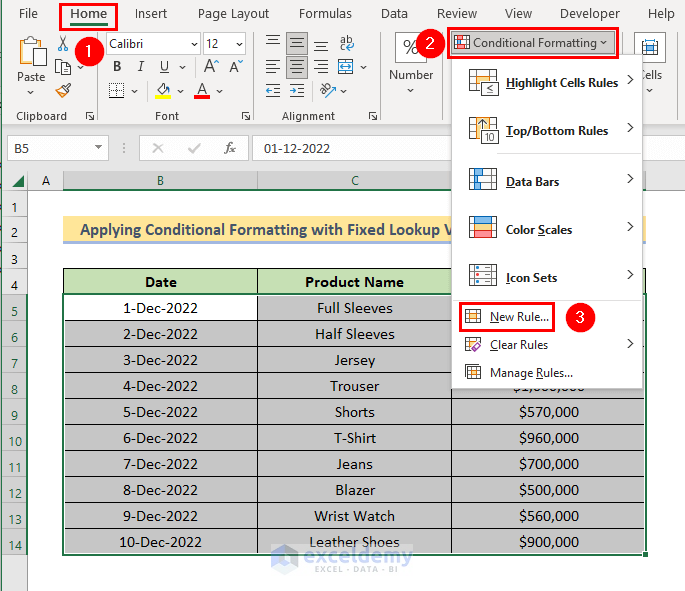
- Go to the Home > Conditional Formatting>New Rule tool in the Excel Toolbar.
- You will see a dialogue box called New Formatting Rule appeared.
- Select use a formula to determine which cells to format.
- Insert any of the following formulas in the formula box:
=D5>INDEX($B$5:$D$14,MATCH("Jersey",$C$5:$C$14,0),3)Or
=$D5>INDEX($B$5:$D$14,MATCH("Jersey",$C$5:$C$14,0),3)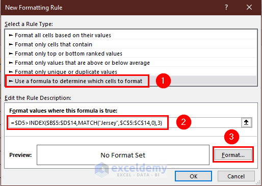
- Click on Format. A dialogue box called Format Cells will appear.
- Choose any format you want to apply to the cells that fulfill the criteria. We chose the light brown color from the Fill tab.
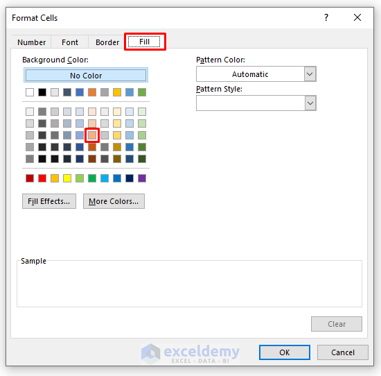
- Click on OK. You’ll be directed back to the New Formatting Rule box.
- You will see a preview in the New Formatting Rule dialog box. Click OK to close the box.
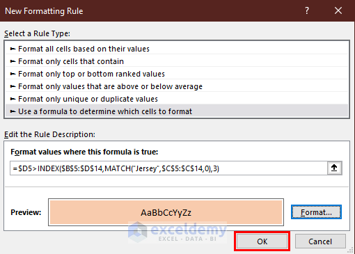
- you will find the names of the products with sales greater than Jersey’s highlighted in light brown.
Formula Breakdown:
- MATCH(“Jersey”,$C$4:$C$13,0) searches each row of the column C5:C14, and returns the number of the row if it finds “Jersey”. See the MATCH function for details. Here it finds “Jersey” in the 3rd row. So it returns 3.
- INDEX($B$5:$D$14,MATCH(“Jersey”,$C$5:$C$14,0),3) now becomes INDEX($B$5:$D$14,3,3). It returns the value from the 3rd row and 3rd column of table B5:D14. See the INDEX function for details. This is the total sales of Jersey, $830,000.00.
- $D5>INDEX($B$5:$D$14,MATCH(“Jersey”,$C$5:$C$14,0),3) now becomes $D5>830000. It returns TRUE if the value in cell D5 is greater than 830000, otherwise, it returns FALSE.
- Now, the formula will move to the next cell of the selected column, to cell C6. It will return TRUE if the value in column D6 is greater than 830000, otherwise, it will return FALSE.
- Move to all the cells from C5:C14 and return TRUE if the value in the respective cell in D5:D14 is greater than 830000; otherwise, it will return FALSE.
- The cells that got TRUE will be highlighted in your desired format, the products that had sales greater than the sales of Jersey will be highlighted.
Things to Remember:
- Here we’ve applied the formula on a single column, that’s why we had to use either the Relative Cell Reference or the Mixed Cell Reference of the cell D5 (D5 or $D5).
- When the formula moves down to cell D6, the cell reference in the formula automatically becomes D6 if you use D5 or $D5. But it would have remained D5 if you had used $D$5 or D$5. (Similar to dragging the Fill Handle with a formula).
- Therefore, while applying Conditional Formatting on a single column, you must use either the Relative Cell Reference or the Mixed Cell Reference of the cells of that column.
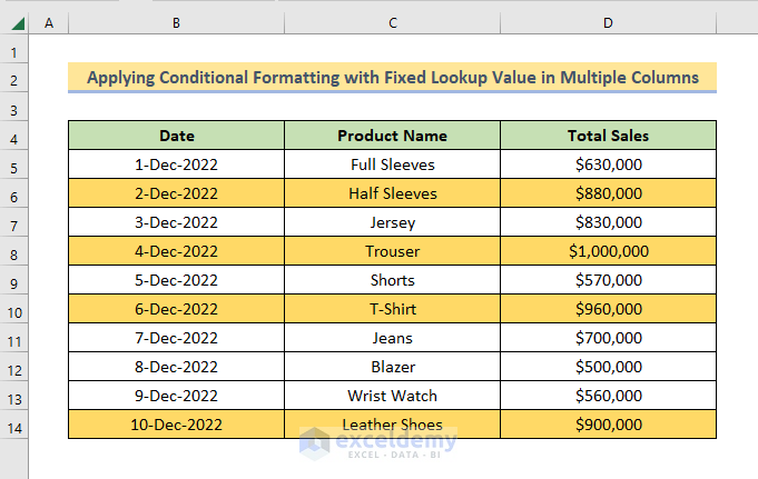
Method 2 – Applying Conditional Formatting with INDEX-MATCH with a Fixed Lookup Value in Excel (Over Multiple Columns)
Steps:
- The steps are the same as the initial steps of Method 1. Just select the whole data set in lieu of a single column.
- Insert the formula with the Mixed Cell Reference.
=$D5>INDEX($B$5:$D$14,MATCH("Jersey",$C$5:$C$14,0),3)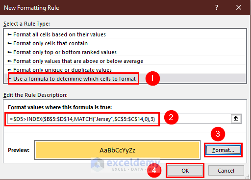
- Choose your desired format from the Format Cells dialogue box.
- Click OK twice. You’ll find the rows with products whose sales were greater than Jersey’s marked in your desired format.
Formula Breakdown:
The explanation of the formula is the same as the earlier method. See it for details.
Things to Remember:
- We applied Conditional Formatting on multiple columns. We used the Mixed Cell Reference of cell D5 ($D5) in the formula.
- When the formula moves to cell B6 from B5, the cell reference becomes D6 from D5, but when the formula moves to C5 from B5, the cell reference remains constant at D5 (Like dragging the Fill Handle).
- While applying Conditional Formatting on multiple columns, you must use the Mixed Cell References of the cells.
Method 3 – Assigning Conditional Formatting with INDEX-MATCH with a Variable Lookup Value in Excel (Over a Single Column)
Steps:
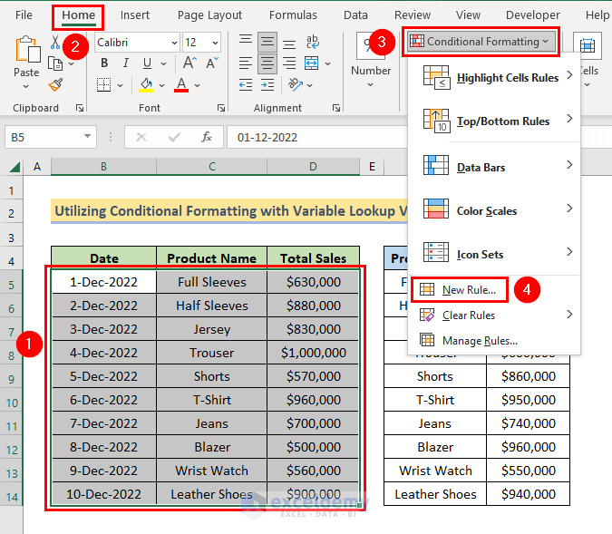
The steps are the same as the previous methods. Select the column Product Name and select New Rule from Conditional Formatting.
- Use one of the two formulas:
=D5>INDEX($F$5:$G$14,MATCH(C5,$F$5:$F$14,0),2)Or
=$D5>INDEX($F$5:$G$14,MATCH($C5,$F$5:$F$14,0),2)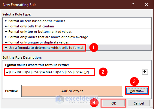
- Choose your desired format from the Format Cells dialogue box.
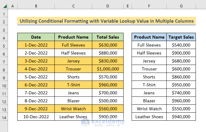
- Click OK twice. The names of the products with sales greater than the target sales will be marked in your desired format.
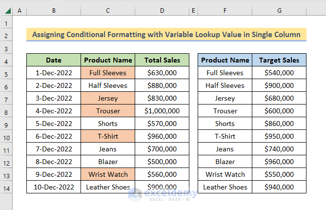
- MATCH($C5,$F$5:$F$14,0),2) searches each row of the column F5:F14, and returns the number of the row if it finds the value in cell C5 there (Full Sleeves). See the MATCH function for details. It finds “Full Sleeves” in the 1st row. So it returns 1.
- INDEX($F$5:$G$14,MATCH($C5,$F$5:$F$14,0),2) now becomes INDEX($F$5:$G$14,1,2). It returns the value from the 1st row and 2nd column of table F5:G14. See the INDEX function for details. This is the target sales of Full Sleeves, $540,000.00.
- $D5>INDEX($F$5:$G$14,MATCH($C5,$F$5:$F$14,0),2) now becomes $D5>540000. It returns TRUE if the value in cell D5 is greater than 540000, it returns FALSE.
- The formula will move to the next cell of the selected column, to cell C6. It will return TRUE if the value in column D6 is greater than 900000 (Target Sales of Half Sleeves); otherwise, it will return FALSE.
- It will move to all the cells from C5:C14 and return TRUE if the respective value in D5:D14 is greater than the target sales, it will return FALSE.
- The cells that got TRUE will be highlighted in your desired format, the products that had sales greater than the target sales will be highlighted.
Things to Remember:
- We applied the formula on a single column, so we had to use either the Relative Cell References or the Mixed Cell References of the cells C5 and D5. (C5 or $C5 and D5 or $D5).
- When we apply Conditional Formatting in a single column, we can use either the Relative Cell Reference or the Mixed Cell Reference in the cells.
Method 4 – Using Conditional Formatting with INDEX-MATCH with a Variable Lookup Value in Excel (Over Multiple Columns)
Steps:
- The steps are the same as Method 1. Just select the whole data set.
- Insert the formula with the Mixed Cell Reference.
=$D5>INDEX($F$5:$G$14,MATCH($C5,$F$5:$F$14,0),2)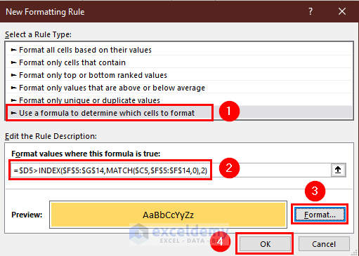
- Select your desired format and click OK twice.
- You’ll find the rows of the products that fulfilled the target sales highlighted in your desired format.
Formula Breakdown:
The explanation of the formula is the same as Method 3. See it for details.
Things to Remember:
While applying Conditional Formatting on multiple columns, you must use the Mixed Cell Reference of the cells.
Download Practice Workbook
you can download the practice workbook from here.
Related Readings
- How to Format Cell Based on Formula in Excel
- How to Use Conditional Formatting Based on VLOOKUP in Excel
- Excel Conditional Formatting Formula with IF
- Excel Conditional Formatting Formula If Cell Contains Text
- Applying Conditional Formatting for Multiple Conditions in Excel
- Conditional Formatting If Cell is Not Blank
- How to Change Text Color Based on Value with Excel Formula
- Conditional Formatting Multiple Text Values in Excel
- Conditional Formatting Entire Column Based on Another Column in Excel
- Excel Highlight Cell If Value Greater Than Another Cell
<< Go Back to Conditional Formatting Formula | Conditional Formatting | Learn Excel
Get FREE Advanced Excel Exercises with Solutions!
